
Fourier Transform
Commonly used spectral analysis method
The Fourier Transform is, by far, the most commonly used spectral analysis method in audio analysis and machine listening. Most of the FluCoMa audio descriptors use this algorithm as the basis of their computation. Because a wealth of resources explaining the Fourier Transform in more general terms already exist, the focus of this resource is going to be on the practicalities of using it within FluCoMa. If unfamiliar with the Fourier Transform or digital sampling, we highly recommend this interactive explanation.
Common Terms and Initialisms
- Fourier Transform: a mathematical operation that decomposes a continuous signal into sine wave components
- Discrete Fourier Transform (DFT): a mathematical operation that computes a Fourier Transform on a discrete signal
- Fast Fourier Transform (FFT): an algorithm for efficiently and quickly computing a DFT on a digital signal
- Short-Term Fourier Transform (STFT): segmenting a signal in to windows and performing an FFT on each window to consider spectral change over time
STFT Parameters
Any FluCoMa object that uses an STFT has three parameters that affect how the STFT is computed: windowSize, hopSize, and fftSize. Each of these is explained more below. Sometimes, adjusting these parameters is necessary to properly analyse a signal (if you’re interested in low frequencies for example), however, changing these can also create different sounding results for many of the algorithms. These three parameters don’t need to be thought of as “set it and forget it”, but instead can explored for the aesthetic differences they might create!
windowSize: The size in audio samples for each analysis window. The default is 1024 samples.hopSize: The number of audio samples between the start of each analysis window.hopSizeless thanwindowSizecreates overlap. The default of -1 indicates thathopSizeshould equalwindowSizedivided by 2.fftSize: The size of FFT to compute for each analysis window. The default of -1 indicates thatfftSizeshould equalwindowSize.fftSizemust be greater than or equal towindowSize. In order to fit the criterial of performing the FFT, iffftSizeis not a power of two, the next largest power of two will be used. For an explanation of settingfftSizegreater thanwindowSizesee oversampling.
Time vs Frequency Resolution
The larger the windowSize, the finer the frequency resolution the FFT provides, however, a larger windowSize also means there is less precision about when the frequency information of the FFT has occurred (because a particular frequency component could be from anywhere within the window). This means that there is a trade-off between the time and frequency resolution of an FFT. A longer windowSize means we are (sort of) averaging information about the signal over a longer time period, but getting more detailed information about the spectrum in return. Correspondingly, a shorter windowSize gives us a better understanding about when-in-time information is from, but a coarser idea about frequency.
FFT Bins per Octave (just in the piano range) for Different windowSizes
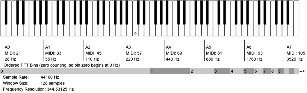
FFT Bins per Octave (just in the piano range) for a windowSize of 128 samples.
As a general principle, if you want to get reliable tracking of partials in a harmonic(ish) sound, you will want to have a conservative 4 frequency bins between partials (because in practice energy gets smooshed across bins). For instance, to reliably identify and track the partials of a sawtooth wave at 100 Hz, you would want a bin resolution of 25 Hz. At a sampling rate of 44100 Hz, this would require a windowSize of 2048 samples (frequency resolution = sample rate / fftSize, or 44100 / 2048 = 21.53 Hz).
For more information about artefacts that can occur because of the Fourier Transform (such as smearing), see the BufSTFT reference.
See this great interactive explanations of time-frequency resolution.
Linear Frequency Scale
The frequencies of the FFT bins that we use are linearly spread from 0 Hz to the Nyquist Frequency (which is often 22,050 Hz). This is strongly mismatched with how humans perceive frequency space: logarithmically. It is important to keep in mind that an octave of pitch space in the low register will have fewer FFT bins per octave than an octave in a higher register, meaning that higher registers are overly represented in FFT analyses.
Bins Per Octave (for the range of the keyboard)
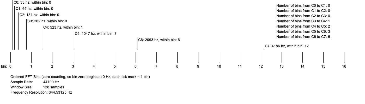
FFT Bins per Octave (just in the piano range) for a windowSize of 128 samples.
One outcome of this mismatch is that, while most of the information humans are perceptually attuned to is below 5,000 Hz, over half of the information provided by an FFT is above 10,000 Hz! (Furthermore, about of a quarter of the information provided by an FFT is in a range most humans can’t even hear!) You might account for this by changing the range of frequencies you want the FFT to analyse. Some objects (such as Pitch and MFCC) take minFreq and maxFreq arguments which allows you to focus the FFT analysis in a register that is meaningful to you. Another approach may be using MelBands which is a further transformation on the magnitudes of an FFT, grouping them into bands that are more perceptually relevant to humans.
Zero Padding and Oversampling
Sometimes using an fftSize larger than the windowSize can be beneficial because it gives us high quality interpolation in the frequency domain frequency because of the “extra” bins we’ve added. In this case, the “added” audio samples used for the FFT are padded as zeros. Note that this does not actually provide higher frequency resolution in the frequency domain. Frequency resolution is still determined by the size of the window being analysed. See Zero Padding for more information.