
Combining FluCoMa with bach
In this article we explore how Olivier Pasquet used the FluCoMa tools to yield artefacts that can be used by other tools such as bach and jtol. The article is accompanied by a series of demonstration patches allowing you to explore the inner workings of the software.
Olivier Pasquet
Introduction
Download the demonstration patches for this article here.
Today we’ll be looking at some of the work that Olivier Pasquet did using the FluCoMa tools. His piece, Herbig-Haro, was performed at the first FluCoMa gig at HCMF 2019. Compared to the other performances – which all featured the musician centre-stage with lights focused on them – his felt much more like an installation. The room was plunged into darkness, Pasquet was barely visible at the back of the stage, discreetly sat behind a laptop. The audience was engulfed in the music: thick bass tones and high, scraping clicks were spatialised across the loudspeakers around the whole performance area; spotlights placed around the space were mapped to flicker on various clicks, pulling the listener into the overarching rhythms that seemed to drive the chaotic material.
At certain points (2:30-4:00, 9:00-9:45 and 10:45-11:20), from this texture there emerged a different kind of material. Strange, filtered voices that seem to teeter along the border of meaningless syllables and textual signification. They are starkly contrasted to the constant gestures of synthetic and electronic basses and clicks – their stumbling between noise and meaning gives them a strangely uncanny, human aura. It seems apparent that they hold a particularly important place in the piece, both structurally and aesthetically. What are these artefacts, and how were they forged?
Pasquet focused a lot of effort into developing a system to create these sounds. He notably took some of the FluCoMa tools and worked them into some of his pre-existing workflows: he makes extensive use of the bach and cage libraries in Max which rely on the lisp-like linked list (llll) data structure; he has also built a library of his own, jtol, which is built around many of the bach objects and deals with real-time pattern generation. In this text we shall explore what Pasquet wanted to achieve with his system and examine how the FluCoMa tools can yield artefacts that can be used by other tools such as bach and jtol. As with all the ”Explore” articles, there is a series of demonstration patches that can be downloaded and interacted with if you wish to explore the inner workings of the software.
The Premise
In his software, Pasquet left an enigmatic Max comment that seems to explain what he was trying to achieve:
Idea: like one sound. Sound as untimed. This gives it timing.
So physical model control is great.
Vocal synthesis is good because low entropy.
Particularly difficult with voice because of the expectation for meaning. This voice in electronic music
Let’s break this down. The first line appears to inform us the most: Pasquet wants to take a sound that would be untimed and give it timing. This suggests to us that a sound in Pasquet’s perspective is a basic unit: a slice that has energetic content, but which has no inherent content in any temporal dimension. In the DSP world, we could think of this as an FFT spectrum of sound. The idea then, would be to take this basic, energetic unit and offer it content across a temporal dimension.
This begs two questions:
First, what does Pasquet consider to be a basic unit, a sound? As we shall see when exploring the software, it isn’t quite as simple as just taking a single FFT spectrum of audio. Indeed, Pasquet makes heavy use of the FluCoMa tools to access a sound, and the way he approaches this gives us an inscribed trace of how he conceives of this elusive notion. Going beyond a simple segmentation of a piece of audio at certain points in time, he levies NMF processing, pitch analysis and onset detection to carefully dissect the audio into much more refined objects.
The second question is how does he give this sound timing? Again, we shall see how Pasquet used the FluCoMa tools in conjunction with bach, jtol and cage to perform this operation. We shall notably try to understand the singular way in which he conceives of an audio file as a collection of sounds, and how the relationships between these sounds can be engaged with to offer them timing.
Finding Sounds
Overview
The sources that Pasquet uses have a very particular nature. In his premise, he tells us that “physical model control is great” and that “vocal synthesis is great because low entropy”. We shall return to these statements and what they mean later; but in the meantime, we can see that this is indeed the type of source material that Pasquet used. A short example can be found below: a short text of vocal sound synthesis, giving a spoken rendition of some somewhat cliché, generic hip-hop phrases. He experimented with 4 different variations of this, all very similar. As a side note, it is interesting to remark the parallels to be drawn between the tropes of traditional hip-hop and the broad structure seen here: electronic, percussion-heavy accompanying music which leaves an important place to unsung, rhythmic vocals.
To find sounds in this audio, Pasquet’s performs the following processes:
- A first NMF decomposition of the audio into 100 components.
- Pitch analysis of these 100 components, and grouping of these components into 10 frequency bands.
- For each of the 10 frequency bands, combining the bases into one combined base for each.
- Using these 10 bases as fixed bases, a second NMF decomposition and resynthesis creating 10 new components.
- Onset analysis of these new components.
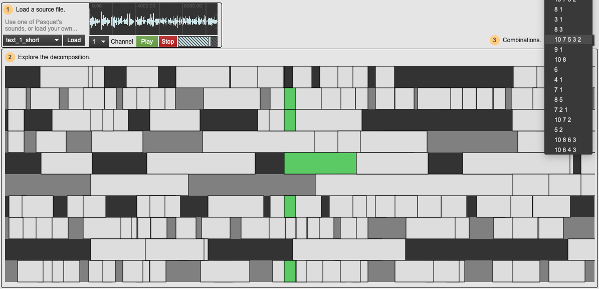
Before breaking down some of these steps, we can gain a better picture of the overall process with a visualisation. The image below is taken from the 01 Finding Sounds example patch. The user has loaded a short piece of audio, each row corresponds to a different frequency band, and each white block an event in this band in time. Note that in dark green, a sound has been selected: the sound deploys itself across 3 different frequency bands (3, 4 and 8), all starting at the same time, but with different durations.
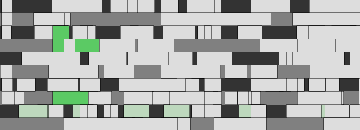
Visualisation taken from the '01 Finding Sounds' demo patch.
Pasquet groups these sounds together so that all the different combinations of frequency bands may be queried together. In light green, we see all the events that are only on the 9th frequency band. These different events, some only in one band, some across multiple bands, are each considered a sound in Pasquet’s sense of the word and shall be the building blocks for his manipulations. Let’s look in more detail at how he gets to these sounds.
Building Grouped Frequency Bands
We’ll first examine how and why Pasquet builds up these frequency bands. As you can see in the image above, there are only 10 different bands. This is quite a low number, especially when compared to something like a traditional FFT analysis to which this process could be loosely assimilated. Each band has a general mean frequency and is filled with parts of the original audio that occupy those fields. This tells us that in Pasquet’s conception of a sound, the range of frequencies that a band will cover is larger than a simple FFT bin and will contain some kind of meaning.
He begins by performing a broad NMF analysis on the audio, asking the algorithm to find 100 components. This is a large number, and as you can imagine, each component is very quiet, with the original audio being quite indiscernible. Pasquet takes these components and groups them together in a way that reveals an organising vector in the constitution of a sound.
He first analyses each of these 100 components by pitch. This process can be viewed in the example patch 02 Pitch Analysis. There are a few elements to note:
- He looks to find the mean pitch for each component across all frames.
- He ignores any frames where the energy is below -60dB.
- He ignores any frames where the pitch confidence is below 0.68.
He is looking to gain a general idea of pitch for each component, but only for frames where he deems the information to be useful. He does not allow frames of silence or frames where the algorithm is not certain there is a pitch to bias his results. This can already be considered a first step of curation.
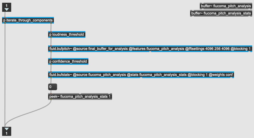
Overview of the pitch analysis process in the '02 Pitch Analysis' demo patch.
Next, he further quantises this information with two steps. First, he rescales the mean pitch for each component. He sees where each of the values will fit in a scale from 1-10. Note that in the overview visualisation there are 10 frequency bands – this is where they are coming from. After this, he groups the components together into these bands.
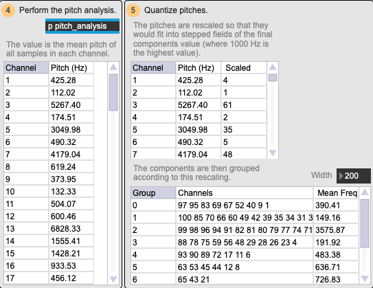
Example of pitch scaling in the '02 Pitch Analysis' demo patch.
Note that when he performs his feature rescaling, he sets the old maximum to 1000 Hz: this essentially means that there will be ten bands going from 0-1000 Hz, and then one band that includes all the components whose mean pitch was above 1000 Hz. This can be seen in the example image above: Group 2 has a mean pitch of 3575.87 Hz, whereas all the other groups have a mean pitch between 0-1000 Hz.
This can inform us about the nature of the sounds in Pasquet’s approach. They are mainly articulated in the 0-1000 Hz range – this is where he differentiates events. Anything above this is grouped together and is considered as one band.
With this information in hand, Pasquet next performs a second NMF analysis. The first analysis was looking somewhat blindly to decompose the audio spectrum into a large number of components. This time, he has a specific idea about what he wishes the algorithm to find. He will give the algorithm a set of fixed bases that are derived from the combinations of bases from the 10 groups of frequency bands: he’s telling the NMF analysis that these are the types of objects to be found in the sound, now find them!
Grouping of the pitch analysis in the '03 Grouped Frequency Bands' demo patch.
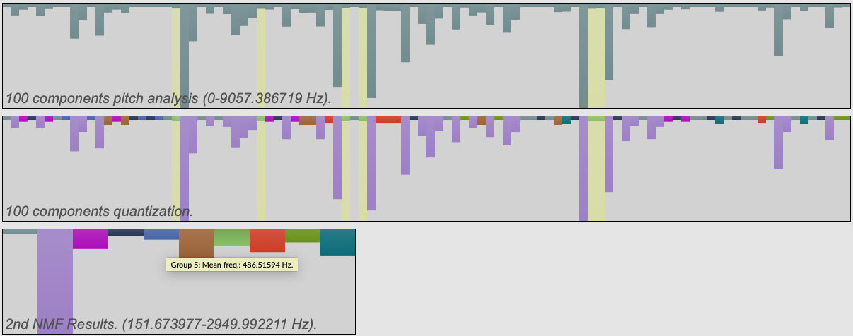
In the example patch 03 Grouped Frequency Bands we see a visualisation of this whole process. Note in the image above how the sound is first decomposed into 100 components and analysed by pitch; then these are scaled and grouped (each colour corresponds to a group); finally, 10 new bases are built (by combining the bases of each component of the same colour) and a second NMF analysis is performed with these 10 bases. In this example patch, you can click on each of the resulting 10 components and hear what they correspond to. In this screenshot, the mouse is hovering over component 5, and the selection of 100 components it is derived from are highlighted in yellow.
We see that in Pasquet’s conception of the sound, we are going beyond a simple decomposition of the audio by pitch. With the second NMF process, we look to find sonorous objects. The search for these objects is guided by the pitch analysis, yielding a result that is much more subtle than a simple grouping of frequency bands.
Finding Sounds in The Bands
Next, Pasquet looks to slice these frequency bands in time to find sounds within them. We begin to understand that the sound in Pasquet’s perspective is something that is inherently tied to perception: we saw with his scaling of the frequency bands into 10 stepped bands, that the organising vectors of difference in pitch need to be broad enough to be perceptibly meaningful. The same will go for slicing in time.
There are two notable steps to discuss: first Pasquet takes each of the bands and runs the FluCoMa onset slicer on them. One notable aspect of this is the way in which he dynamically sets the threshold for each of the bands: he gathers the mean energy description of each of the components and then multiplies this by 0.001. Then, he rejects any slices that are smaller than 200ms.
Finally, Pasquet quantizes the slice data: he rounds the start times and durations of each of the sounds to the nearest 20ms. After this, he groups components that start at the same time together. This is interesting, as it indicates to us that the spectral decomposition of the audio is to be further refined still: if two or more components start at the same time, they are not separate events, they are perceived as being the same event. This means that the range of frequency bands goes beyond the 10 bands that were obtained from the frequency band grouping: we add to this the various combinations of those fields according to activity in the temporal domain.
Overview of the '01 Finding Sounds' demo patch.
In the first example patch 01 Finding Sounds, we can see a list of all these combinations for the processed audio file. In this instance, the user has selected a sound that deploys itself across the 10th, 7th, 5th, 3rd and 2nd frequency bands. They all start at the same time, however, they may not all have the same duration.
In the next section, we shall examine the singular way in which Pasquet stores this information using the bach library, and how he manipulates it using jtol and cage to give these sounds timing.
Timing Sounds
Overview
To begin, let us have a listen to what the results are going to sound like, and discuss the nature of this transformation without delving into the mechanical working of the patch. The example patch 04 Timing Sounds allows the user to load a sound and listen to the final results of the process, comparing the 10 output channels with the 10 components of the second NMF analysis discussed above.
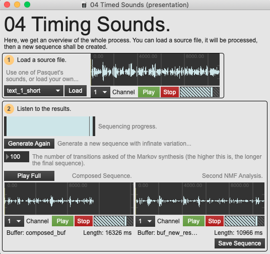
Overview of the '04 Timed Sounds' demo patch.
The sound is notably smeared and various fragments of the original sound are played back in a glitchy manner, seeming to step upon themselves. The source material that Pasquet used is to be taken into account when considering the nature of this tool and its process as they were specifically forged around it. Here, the vocal source is still recognisable and the nature of the original audio is very much present. However, it seems to have been stripped of meaning. We might make out syllables from time to time and disparate phonemes momentarily indicate signification before becoming engulfed within the stream of smeared speech.
Let’s examine how Pasquet arrives at this new sequence. There are two interesting elements to look at: the way in which data is stored, and the way in which data is manipulated.
Storing the Symbolic Data
The analysis examined in the previous section of this text leaves us with a symbolic representation of the audio that is strewn across several different places: the NMF components are stored in a multichannel buffer, the onset information in a coll. In the previous section, we also saw that combinations of onsets starting at the same time in different frequency fields was an important constitutive part of the sound. Where is this information stored? How does Pasquet make this multidimensional data available to the processes he uses for manipulation and sequencing?
As mentioned above, Pasquet makes use of the bach library and the data structure it brings to Max: lisp-like linked lists (lllls). If you wish to learn more about lllls and how they work in Max you can consult the bach documentation. Here it suffices to know that Pasquet uses Bach as a dynamic way of storing and querying data.
There are two primary objects that Pasquet produces to store his data:
- A bach.shelf object which stores lllls. In this, each llll corresponds to one sound in the audio file. This means that they contain information pertaining to the start time, the components, and the durations in each component.
- A large llll which is a list of these sounds. The elements in this llll are the addresses that can be used to query the bach.shelf object to access the corresponding sound. This llll follows the order of appearance of these sounds in the audio file.
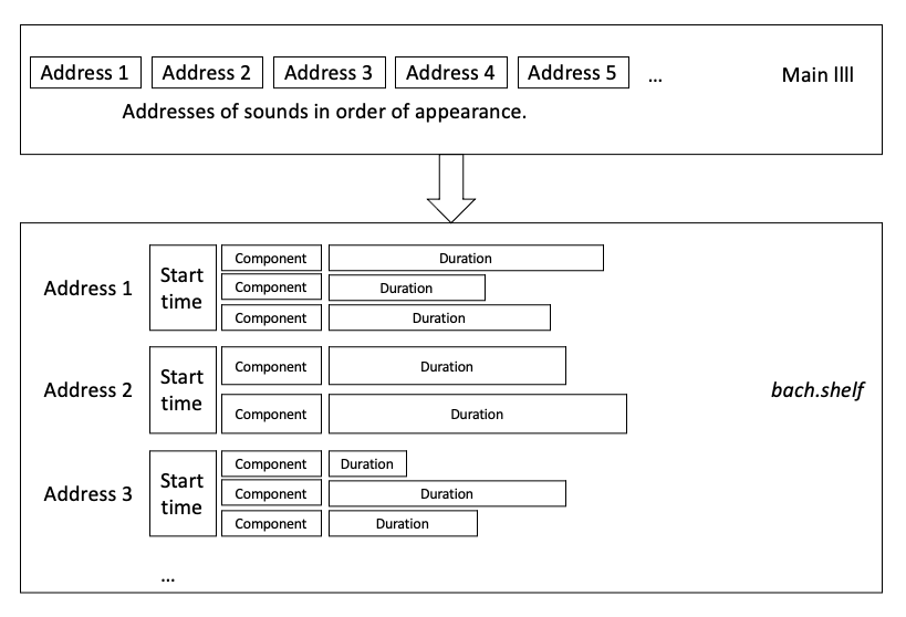
Visualisation of how sounds are stored across various objects.
We can conceive of the first object as the collection of sounds or notes that fill the audio file and the second object as the order in which they are heard. One interesting point to note here: in this symbolic representation, the rhythmic dimension seems to have been left out. Pasquet is primarily interested in the order of events. Thinking back to the premise of the tool, Pasquet announced that he was interested in manipulating sounds. At this point, he has accessed the sounds, and we observe that the internal rhythmic structure of the original audio file is not a concern that he chooses to engage with. The dimension that he retains is the order in which they appear.
This suggests then that to time a sound, Pasquet engages with the context within which it is heard. The sound is the basic sonorous unit, and to time it is to manipulate the context it finds itself in, to manipulate what happens before and after it. Pasquet remarked that this is “particularly difficult with voice because of the expectation for meaning”: the voice is composed of sounds and their combination, their timing, is very important and rigid when we wish to convey meaning with them. Let’s have a look at the way in which Pasquet times these sounds.
Manipulating the Audio File
Pasquet uses the cage implementation of Markov chains to manipulate the relationships between sounds. If you wish to learn more about Markov chains, you can have a look here. Here, it is enough to understand that Markov chains will make decisions about sequential information based on a model - it is a way of describing the probability of moving from one ‘state’ to another (where a state may be a musical decision such as a section, sample, note, parameter or chord). The model that Pasquet supplies here is the large llll that contains the order in which sounds appeared in the original audio file.
He first compresses this data using his implementation of the ”Lempel-Ziv-Welch” compression algorithm. This is a data compression algorithm that essentially works by finding repeated patterns in the original data and creating a mapping of keys corresponding to these patterns. This allows the data to be represented with less characters, and can be decrypted with the key mapping when we want to decompress it.
After this, he derives from this compressed data a Markov transition matrix (this is what the markov chain algorithm uses to make decisions). He then creates a new sequence of sounds that use this transition matrix as their model. Essentially, as Pasquet explains, he can “extend pseudo-repetitive sequences [that were] observed in the initial sequence”. When creating a new sequence, he wishes to retain some of the nature of the original model. The sequence is then decompressed and played back according to this new sequence. The result is a sequence of sounds that have gained new timing, something that is particularly striking when applied in this context to the voice.
Conclusion
Let’s return to the initial premise that Pasquet announced. We have seen how Pasquet used the FluCoMa tools to extract sounds from an audio file, and how he used the bach and cage libraries to extract sequential information about these sounds and manipulate it to grant these sounds timing.
He also stated that “physical model control is great” and that “vocal synthesis is good because low entropy”. We understand this as being tied to the LZW encoding process. When explaining this process, Pasquet discusses the notion of the “variety of scales” where the smallest units retain their identity. He explains that the low amount of entropy in speech allows for easier identification of smallest units that retain identity (essentially syllables), and thus proposes it as a good candidate for this kind of approach. We see then that Pasquet’s sound, in the context of speech, is the smallest unit that retains identity, that retains meaning.
His use of the FluCoMa tools can be seen as a way of decomposing audio not into incomprehensible elements that have meaning only for the algorithm that created them, but into units that retain identity, that retain signification, that are perceived by humans as sounds. He uses the tools to draw the distinction between the decompositions that computational techniques allow us to perform on audio into microscopic elements, and decomposition into smallest elements that mean something. He demonstrates that machine learning can be configured in a way that yields something inherently human.