FluCoMa and Musicological Analysis
In this article we take a look at how Jacob Hart used some of the FluCoMa tools for musicological analysis.
Jacob Hart
Introduction
Download the demonstration patches for this article here.
This article will differ slightly from others in the ”Explore” collection as it does not focus on the work of an artist that was made using the FluCoMa tools; instead, we shall be discussing some of the work by the author of these articles. I shall be presenting a short autoethnographic account of some of the musicological analysis I performed using the FluCoMa tools during my PhD research. I joined the FluCoMa project in 2018 as a PhD researcher (under the supervision of Frédéric Dufeu and Owen Green), and my task was to track the creative process of the techno-fluent composers who were each commissioned to make a piece using the tools. My approach led me to use computational techniques for my analysis, and to use some of the FluCoMa tools and related technologies extensively. As with all the ”Explore” articles, there is a series of demonstration patches that can be downloaded and interacted with if you wish to explore the inner workings of the software.
A presentation I gave on the state of my research at a FluCoMa plenary in 2019.
As per tradition, my research was bound within a written document called a doctoral thesis that was entitled: Performance cartography, performance cartology: musical networks for computational musicological analysis. It was also accompanied by an extensive set of digital elements which included software, audio, video, images, and many bespoke elements such as interactive network graphs and performance recreation systems. Today I will begin by giving a brief overview of the theoretical context my research emerged from. Then, I shall present some of the techniques I deployed using the FluCoMa tools and related technologies in the goal of tracking the creative process of a cohort of 9 creative coders and developing my theoretical ideas.
Cartography and Cartology
At the heart of my approach is a conception of music which subscribes to contemporary perspectives entwined within the works of people like Christopher Small, Georgina Born, Carloyn Abbate, Nick Cook and Kofi Agawu. Essentially, I consider musical practice not as a singular object or entity, but as the configuration of networks of entities, and the existence within these networks. I subscribe to Small’s conception of musicking – where musical practice is an activity, something that emerges from engaging with people and things in a musical way. This kind of perspective moves away somewhat from more traditional approaches to musicology, notably away from an obsession with fetichised objects such as the score (this becomes but one object amongst many), and from the despotic figure of the composer (they become but one actor amongst many).
The network approach to the social is not a novel idea: this is a question that has been developed by many. We can cite people such as Latour and Callon and their Actor-Network Theory or Tim Ingold and his meshworks in a broader sociological context. In musicology this kind of approach has been developed also, for example by Benjamin Piekut in a historical context, and Thor Magnusson in an organological one. Indeed, to regard musicking as the configuration of networks is to adopt a characteristically organological approach, and my goal was to put this kind of perspective to the service of a more aesthetic analysis of the creative processes that the composers on the FluCoMa project presented.
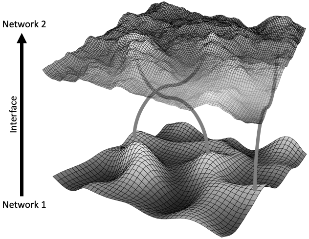
Illustration of the idea of network superposition, developed in the PhD.
This was articulated through three primary research interests. First, I wished to develop the notion of time in a network approach: rather than regarding one temporal occurrence to emerge from a musical network, I wished to try and gain access to the entire scope of potentialities a network could allow. Next, I wished to explore and develop the idea that an artist’s musical thought (an inherently intangible concept) may become somewhat inscribed, materialised within the physicalities of a network. Finally, I wished to explore the idea of interface, and points of interface within a network (and between networks) as being particularly rich zones of aesthetic activity.
If you are curious to learn more about these ideas, they are of course developed in much more detail in my PhD. Today, we shall specifically be looking at some of the methods and digital tools I created in order to cater to some of these ideas.
Data Navigation
I shall distinguish two main uses that I make of computational techniques regarding their relationship with data: the navigation of data and the creation of data. I argue that, when computational techniques have been used in musicology before, it is usually for the navigation of data. One popular example of this are the numerous studies we see of large datasets of musical metadata which tend to focus on questions around listening practices and the classification of musics around genres. Another is the use of spectrograms for musicological analysis: instead of referring to a score, we can use spectrograms to illustrate much more granular concepts pertaining to things like timbre.
The computer gives us the power to explore very large amounts of data. Indeed, as you can imagine, over the course of my ethnomusicological research, I gathered huge amounts of data of various types: audio, video, images, text, code. A primary use of computational techniques is the ability they offer us to navigate these large collections of data in ways that would otherwise be impossible – this is one of the founding premises of machine learning and is also at the heart of the FluCoMa project. Computational techniques seek to respond to the problem that computers have created: access to collections of overwhelming amounts of information.
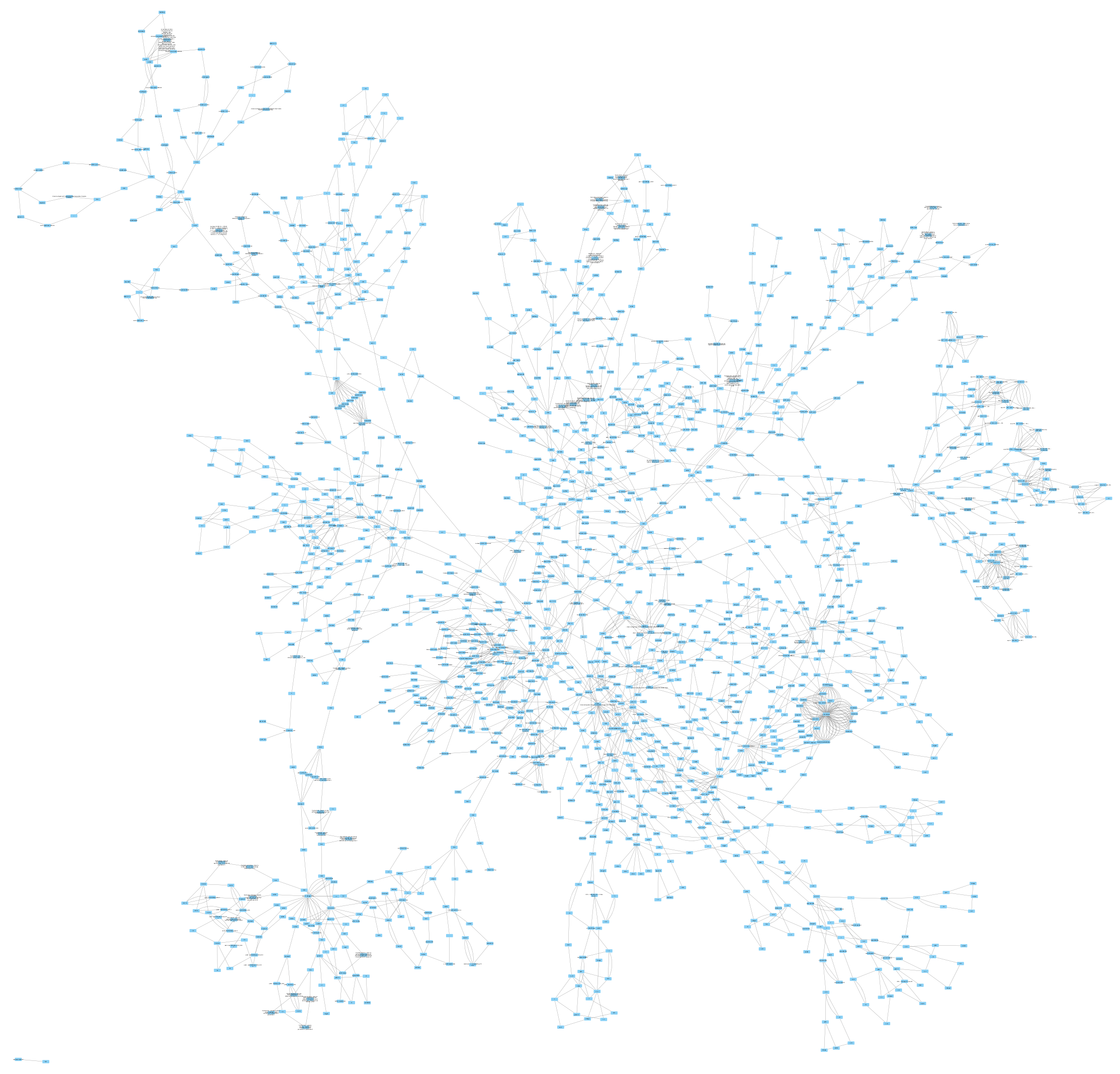
Network visualisation of a Max patch using a prefuse force-directed layout algorithm.
One way in which this was useful for me was to create interactive network visualisations of the physical networks of entities that the artists configured. I did this using a pre-existing piece of software initially designed for biologists called Cytoscape. I was able to create dynamic networks at various levels: global levels that revealed the agency of various institutions in the artists’ work; local levels around the FluCoMa project and how different people could influence each other, and instrumental levels, where each component of an instrument was represented in a very detailed manner. I also developed a tool in Python which would allow me to translate entire Max patches into network form and insert them into networks representing the physical objects and spaces they were connected to and inspect the relationships between them.

Visualisation of a Max patch using a radial layout algorithm.
Computational techniques allowed me to navigate these networks in intelligent ways. I could use automatic layout algorithms and dimensionality reduction to display the networks in different ways that could reveal aspects about its inner structure, I could filter nodes in and out, follow paths of edges of different types to follow energy as it travelled through the network and was translated by different elements. This allowed me to gain a better understanding of the structure of the network each artist was configuring, rather than just the sonorous aspect to emerge from it at one point in time.
Very pragmatically, the FluCoMa tools allowed me to make sense of large amounts of data without losing inordinate amounts of time. A concrete example of this is discussed in my article on Richard Devine’s work for the project and can be examined in the example patch 01 Source Navigation. In this patch, as explained in the video above, I wanted to find a solution to the following problem: given two datasets, one very large one of lots of diverse samples, and another of three ‘reels’ which were used for a performance, comprised of slices from the samples; how can I discover which samples were used to make each reel? Of course, it would be possible to manually go through each reel, and each sample – however this would be extremely tedious, and highly subject to human error.
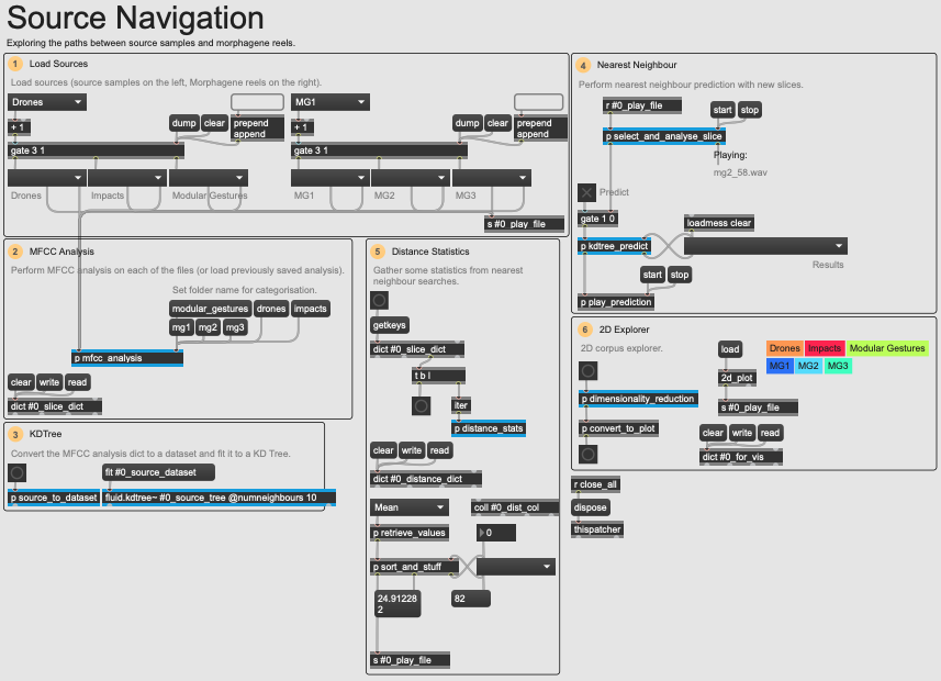
An overview of the 01 Source Navigation example patch.
To respond to this task, I made this patch which performs an MFCC analysis on each of the two datasets, and performs nearest neighbour searches using fluid.kdtree~. Not only did this allow me to very quickly discover which samples were used to make up each of the reels, but also perform statistical calculations and rankings which allowed me to discover for example that one reel tended to use exact copies of samples, whereas another would combine parts of different samples and so on.
This kind of process is extremely useful for musicologists, and especially ethnomusicologists who find themselves dealing with large amounts of data. However, for me this only scratches the surface of what computers may offer as bespoke tools for analysis. Let us now take a look at the second aspect mentioned above: that of the creation of data.
Data Creation
One of the research questions I mentioned above was that of time in the network-driven approach, and the will to gain access to the entire scope of potentialities of a network. In my musicological context, a natural inflection of this goal is to gain access to the entire scope of sonorous potentialities of an instrument. This is where computational techniques can help us again, especially in the case of networks where a large part of activity occurs in the digital domain, as we can envisage automated recreation of performances and the creation of data to conceptual infinity.
There are several possible approaches to this idea. All begin with a process of faktura as described by Marc Battier and Olivier Baudouin. This is a method for analysis of code and digital music systems which consists of three steps: transcription (an accurate recreation of the original code); concordance (checking that this code produces results as similar to the original as possible); and exploitation. To these first two steps I also add the idea of factorisation: often (although not always, see Rodrigo Constanzo) artists will code quickly and without particular care for optimization and things like commenting. Although it is important to bear in mind during analysis when these aspects become integral aspects of the piece, it is also useful and important to factorise the code, make things as tidy as possible, and gain a good abstract image of how the various pieces fit together.
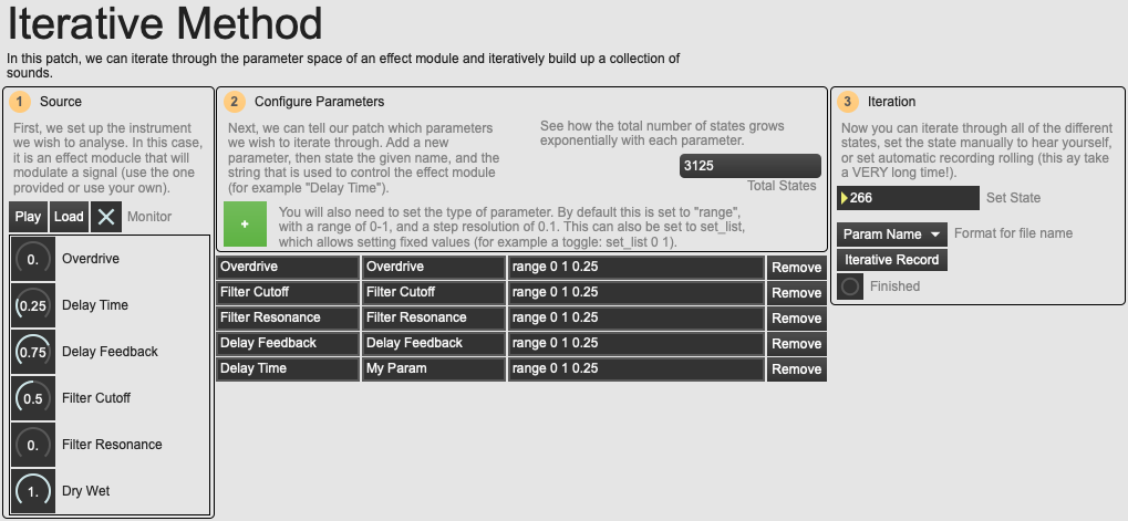
An overview of the 02 Iterative Method example patch.
Once these steps are accomplished, exploitation may occur in analytical conditions where the musicologist has complete control over any number of parameters they may be interested in. My first approach to accessing the entire scope of sonorous potentialities of an instrument was to, somewhat heavy-handedly, iterate through the entire possible parameter space of an instrument. This is demonstrated in the example patch 02 Iterative Method. This comes with several drawbacks:
- It is in fact impossible to access every configuration of a parameter space if there are analogue, continuous parameters involved (for example, a slider between 0. and 1.). It is therefore necessary to define a resolution for analysis which will greatly affect the number of possible configurations.
- The sum of possible states of a parameter space is a cartesian product, and as such this number can grow very quickly to extraordinary numbers.
- As we shall explore further below, this method is somewhat reductive in regard to the complexity of an actual instrument, and in some cases will make no sense at all. It is therefore a method that is difficult to generalise.
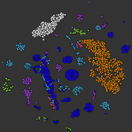
A 2D distribution (see below) of the output of iteration over the various effect chains in Rodrigo Constanzo's network.
This is a method I tried when analysing Rodrigo Constanzo’s work (see the article about his piece here). Indeed, as I explain in that article, his patch was configured around a number of effect module chains, and it was possible to iterate through their different states to a certain extent. This method did shine light on some interesting ideas regarding the nature of the network, however it soon became clear that this method was far from optimal.
Another method which seems to hold more promise is that of alternative performances. This itself can have various forms. The first is taking recordings of previous or subsequent performances – be they in a concert setting or in rehearsal/over development. This was something I tried with Lauren Sarah Hayes’ work (see the article on her piece here) who was kind enough to provide me with several hours’ worth of audio recordings of her rehearsals. Again, sifting through such quantities of audio manually is an unsatisfactory solution: I turned to the FluCoMa tools for help.
At the second FluCoMa plenary back in 2019, I was struck by a project that one of the team members presented: Gerard Roma presented a 2-dimensional sound plot where each point corresponded to an audio file. The sounds were distributed in the space according to an MFCC audio description and dimensionality reduction. This technique is now a somewhat of a characteristic use of the FluCoMa tools – consult the video tutorial above – however, at the time it was a fairly new concept for me, and I was instantly inspired.
There are three main issues to think about when approaching the construction of a 2-dimensional corpus explorer, be it from a compositional or analytical point of view:
- Slicing: the way in which the target we wish to explore will be segmented. Sometimes this is self-evident, other times it is something that will be in itself an active act of analysis.
- Description: what is the way in which we shall describe the audio in order to obtain information and distributions that will make sense and that will be useful for analysis.
- Distribution: how will the information be conceived of and distributed across the 2-dimensional space: essentially, which dimensionality reduction algorithm (if any) should be used?
When looking at Lauren Sarah Hayes’ work, slicing was a question that I chose to approach using the FluCoMa tools. The type of audio (listen above to some extraits) was very diverse, and there was a lot of it – therefore it seemed that neither transient nor onset detections would make sense. The perfect tool for this was FluCoMa’s fluid.bufnoveltyslice~ object. This could be set to something like the MFCC feature, and look for differences in this, rather than the beginning of events. Experimenting with various settings such as different FFT settings, different thresholds and different kernel sizes allowed me to get a segmentation that, while not perfect, was good enough for analysis. Indeed, the criteria and needs for the analyst can be lower than those of the artist.
That being said, there are more satisfactory ways of approaching slicing. For example, in the case of my analyses of Leafcutter John’s work and Olivier Pasquet’s work, I was able to configure entire performances in analytical conditions and could define the slicing of the audio while these performances were playing out. This has the advantage of not only giving a segmentation that makes sense, but also of inherently inscribing an aspect of the network’s nature and structure within the slicing. If the network we are dealing with allows for this kind of alternative performance creation, as was the case with Pasquet and Leafcutter John’s work, it is preferable to dissect one’s sources while they are being collected. It is also good practice to keep audio streams separate and to gather more information than one needs rather than regret not having something later on!
2 and a half hours of alternative performances of Leafcutter Johns system.
This type of source collection and creation can continue as long as we wish depending on the kind of things we wish to examine in the network. I found that it was important to perform an initial analysis of the physicalities of a network beforehand so that my alternative performances may be guided and grounded in reality. Once the sources are collected and sliced, we can use audio descriptors and dimensionality reduction to organise them into a 2-dimensional space.
I experimented with many different kinds of combinations of descriptors, dimensionality reduction algorithms and settings. As the corpora are generally large, a good initial description is using MFCC (especially if the slicing was performed automatically with fluid.noveltyslice~ using the MFCC feature). As analysis continues, and one gains a better sense of the corpus, it is possible to make subcollections and to use other audio descriptors. Dimensionality reduction was also a very important aspect: at the time I was carrying out this research, only the fluid.pca~ and fluid.mds~ objects were implemented in the toolkit, and I found them to yield unsatisfactory results. Therefore I exported my analyses from Max and used a Python patch (see below) built around scikit-learn to build distributions which could then be opened again in Max.
'''
---- Other reductions ----
With this script, we can take a standardized corpus description exported from the "03 Corpus Exploration"
Max patch, and use scikit-learn to perform some other dimensionality reductions.
Set the output folder to the place that you saved the PCA, MDS and UMAP reductions from the Max patch.
The reductions will be saved to this folder, and will then be able to be loaded back into the patch
for interation.
'''

import os
params = { # Set the source file, output folder and file prefix here:
    "corpus_description_file" : os.path.join(os.getcwd(), 'data_reductions/high_res_desc.json'),
    "output_folder" : os.path.join(os.getcwd(), 'data_reductions'),
    "output_file_prefix" : 'High Res Example'
}

import json
import numpy as np
from sklearn.manifold import TSNE
from sklearn.preprocessing import MinMaxScaler
from sklearn.manifold import Isomap
from sklearn.manifold import LocallyLinearEmbedding
from sklearn.manifold import SpectralEmbedding

def process():
    original_data = load_json(params["corpus_description_file"])
    np_data = convert_to_np(original_data)

    print('T-SNE Processing...')
    tsne_data = process_tsne(np_data)
    export_data(original_data, tsne_data, 'tsne')

    print('Isomap Processing...')
    isomap_data = process_isomap(np_data)
    export_data(original_data, isomap_data, 'isomap')

    print('Locally Linear Embedding Processing...')
    lle_data = process_lle(np_data)
    export_data(original_data, lle_data, 'locally_linear_embedding')

    print('Spectral Embedding Processing...')
    spec_data = process_spec(np_data)
    export_data(original_data, spec_data, 'spectral_embedding')

def load_json(path):
    f = open(path)
    data = json.load(f)
    f.close()
    return data

def write_json(data, path):
    with open(path, 'w') as outfile:
        json.dump(data, outfile, indent = 4)

def export_data(slice_data, reduced_data, type):
    to_export = {
        "cols" : 2,
        "data" : {}
    }

    count = 0
    for item in slice_data["data"]:
        to_export["data"][item] = reduced_data[count].tolist()
        count = count + 1

    write_json(to_export, os.path.join(params["output_folder"], params["output_file_prefix"] + "_scikit-learn_" + type + '.json'))

def convert_to_np(data):
    global_array = np.array([])
    for item in data["data"]:
        this_array = np.array(data["data"][item])
        if np.size(global_array) == 0:
            global_array = np.append(global_array, this_array)
        else:
            global_array = np.vstack((global_array, this_array))

    return global_array

def process_tsne(data):
    tsne = TSNE(n_components = 2)
    reduced = tsne.fit_transform(data)
    normed = min_max(reduced)
    return normed

def process_isomap(data):
    iso = Isomap(n_components = 2)
    reduced = iso.fit_transform(data)
    normed = min_max(reduced)
    return normed

def process_lle(data):
    lle = LocallyLinearEmbedding(n_components = 2, method='standard')
    reduced = lle.fit_transform(data)
    normed = min_max(reduced)
    return normed

def process_spec(data):
    spec = SpectralEmbedding(n_components = 2)
    reduced = spec.fit_transform(data)
    normed = min_max(reduced)
    return normed

def min_max(data):
    scaled = MinMaxScaler((0.1, 0.9)).fit_transform(data)
    return scaled

process()
I experimented with many algorithms: pca, mds, umap, t-sne, self-organising map, isomap… I am primarily a musicologist, and I admit openly that I have very little idea about how these algorithms actually work. What interests me most is the artefact they deliver, and in order to explore these fluidly I created an exploration patch (see example patch 03 Corpus Exloration) which allowed me to quickly and dynamically explore and interchange different distributions. Each have their own caracteristics, and yield different types of documents. For my uses, I found t-SNE and umap especially effective (especially umap which has now been implemented in the toolkit with fluid.umap~). These were most useful as they often yielded distributions which were somewhat even across the 2-dimensional space and offered clusterings that were easy to read.
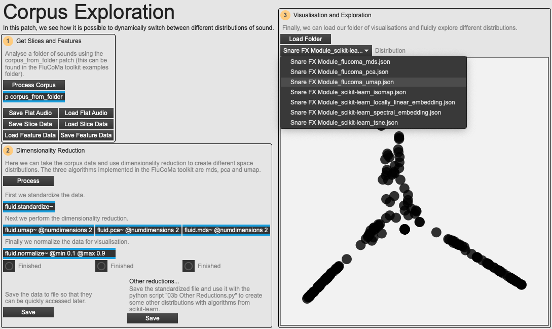
An overview of the 03 Corpus Exploration example patch.
These processes allowed me to see and fluidly explore how the networks in question could have sounded out – it is of course impossible to access the entire scope of sonorous potentialities a network can offer, but this allows us to gain a very well-informed image. Things become even more interesting when we append to these networks slicings of performances from the night, or sample libraries used within the network. We can observe which extremes of the sonorous potential the musician opted to explore during performance, and which they left aside; we can see how sounds have been transformed from source to performance. It is even possible to recognise more macroscopic structures: for example, I would often find distributions where there would be one large cluster of sound morphological profiles, and generally one or two others. This can suggest the grounded, basic sound world the creative coder implemented, and then the tangents away from that they would push the system into. Naturally, there is not enough time here to recount the details that this kind of analysis can provide, but we begin to see that the use of these computational techniques can yield very interesting results.
Conclusion
This is somewhat of a new step in musicology (although I am by no means alone in this kind of research, see Frédéric Dufeu, Michael Clarke, Thor Magnusson, Pierre Couprie, or Clarisse Bardiot among many others). As we move away from traditional methods, we must be wary of charging ahead without addressing some of the issues that arise. In this case, we see a curious situation where, not only is the focus of the analyst shifted away from the traditional subject of analysis (this is characteristic of a recent turn in musicology to focus on other artefacts that bear trace of the creative process: sketches, instruments, code etc.); here, the analysist now puts themselves into an attitude of active creation of artefacts that shall then become a subject for analysis. Is this moving too far from reality?
I should like to think not – in fact I would even argue that this can shed a brighter light on reality, in as much as we gain a better understanding of the system, the network from which the musical practice emerged (in accordance with the perspective on musical practice I announced at the beginning). Does this analytical practice take away from, or fail to appreciate the wonderous aspect of that very moment in the concert? Again, I think it does the opposite: in understanding the infinite variation that could have occurred, the precise and shared moment of performance gains even more wonder in our mind. Out of everything that could have happened, out of everything the musician made possible in the configuration of their network, this moment emerged at the crossroads of them, and us.
