Neural Network Parameters

by Ted Moore

A guide on using the parameters of and MLP.

This article provides guidance on using the parameters of the neural networks found in the FluCoMa toolkit. FluCoMa contains two neural network objects, the MLPClassifier and MLPRegressor. “MLP” stand for multi-layer perceptron, which is a type of neural network. “Classifier” and “Regressor” refer to the task that each MLP can be trained to do. For a deeper understanding of how the MLP training process works, visit MLP Training.

Parameters

hiddenLayers

A list of numbers that specifies the internal structure of the neural network. Each number in the list represents one hidden layer of the neural network, the value of which is the number of neurons in that layer. For example, 3 3 (which is the default) specifies two hidden layers with three neurons each. The number of neurons in the input and output layers are determined from the corresponding datasets when training begins.

When deciding what the internal structure of your neural network should be, a good place to begin is using one hidden layer with a number of neurons between the number of inputs and the number of outputs creating a “funnel” shape (if using MLPClassifier, the number of outputs is the number of classes). For example, if my neural network is taking in 13 MFCCs as the input and 3 synthesis parameters as the output, starting with one hidden layer of 8 (right in the middle), would be a good place to start.

If the neural network is not learning as well as you would like it to, you may consider adding more neurons to this single hidden layer. If it is still not learning, you might add some more layers (again considering the funnel shape). If it is still not learning how you would like, it may be the case that your data doesn’t have strong enough patterns for the MLP to learn!

Because changing hiddenLayers changes the internal structure of the neural network, the internal state of the neural network is necessarily reset and any training that has been done will be lost. Even so, it is a good idea to play with this parameters because it can have a significant impact on how well and how quickly the neural network is able to learn from the data.

Total Number of Internal Parameters

Generally speaking, the larger the internal structure of a neural network is, the more data points it needs to train. A general-principle is to have about ten times as many data points as there are the total number of internal parameters. The number of internal parameters in a neural network is total number of weights + the total number of biases. The total number of weights equals the sum of the products of each pair of adjacent layers. The total number of biases is equal to the number of hidden neurons + the number of output neurons.

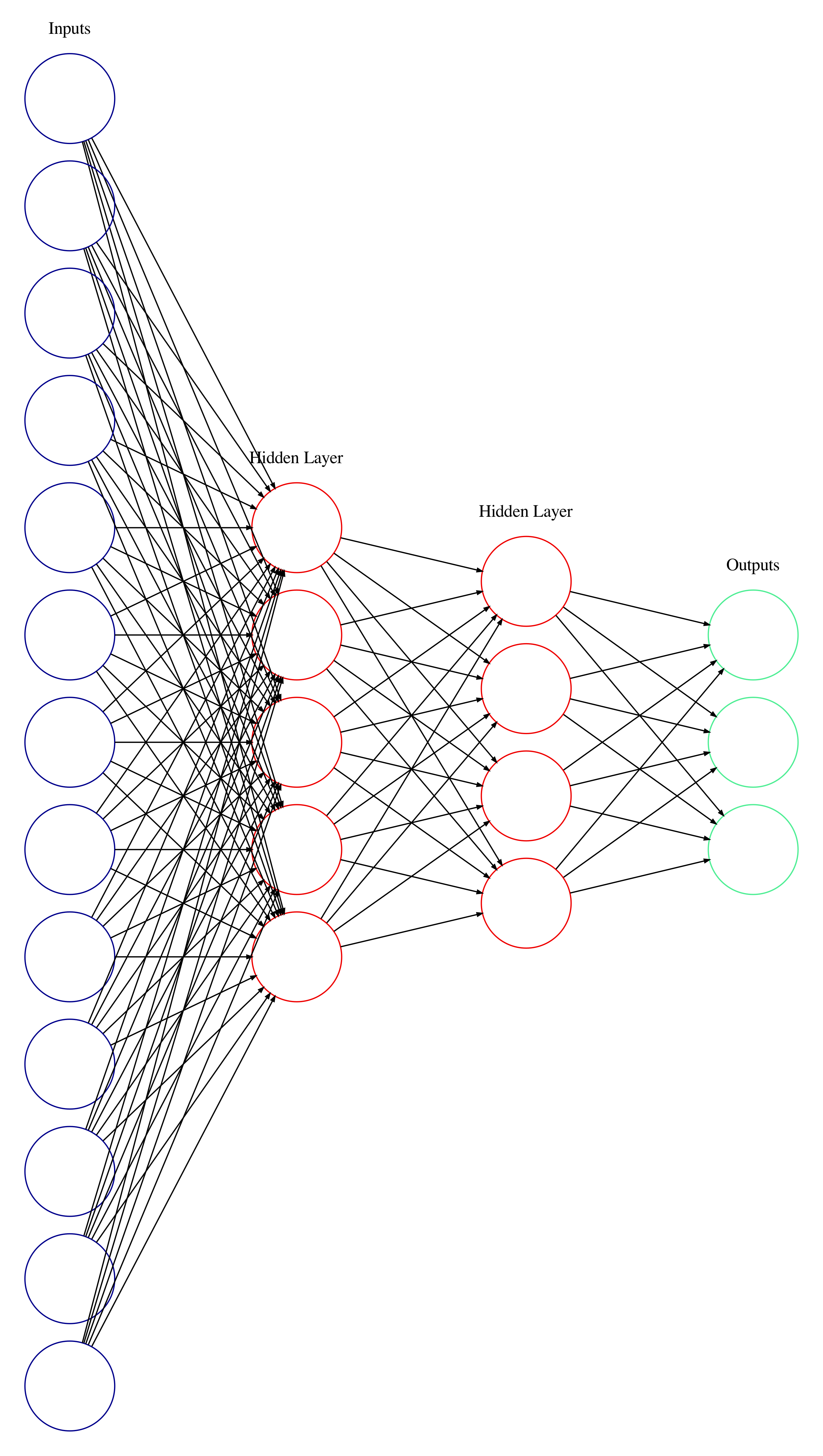
For example, consider a neural network with 13 input neurons, two hidden layers of 5 and 4 neurons, and an output layer of 3 neurons. The total number of weights is ( 13 * 5 ) + ( 5 * 4 ) + ( 4 * 3 ) = 97. The total number of biases is 5 + 4 + 3 = 12. Which makes the total number of parameters 97 + 12 = 109. The general-principle suggests that it would be good to have around 1,000 data points (about ten times as many) to successfully train this neural network. In practice, a neural network of this size may be able to learn from many fewer points. It completely depends on how clearly patterns in the data are represented. This general-principle may become important if your training is not going well—consider how many point you have and how that compares to how many internal parameters are in your neural network. Based on these numbers consider changing the size of your neural network or using a different number of data points and see if your neural network improves.

Activation Functions

• The MLPClassifier has the parameter activation
• The MLPRegressor has the parameters activation and outputActivation

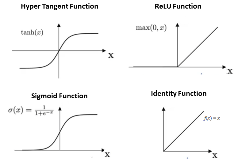
activation is an integer indicating which activation function each neuron in the hidden layer(s) will use. The MLPRegressor has the additional parameter outputActivation, which uses the same set of integers to specify an activation to be used in the output layer of the neural network. Each neuron in the hidden and output layers processes its output by the activation function before it is passed along to the next layer. These activation functions are non-linear functions (except for “identity”) which allow the neural network to learn non-linear relationships between the input and output data. Each of the activation functions transform values in different ways and will create different training processes, learned mappings, and output predictions in a neural network, so they all may be worth trying during training to see what creates the best result.

Because changing activation or outputActivation changes the internal structure of the neural network, the internal state of the neural network is necessarily reset and any training that has been done will be lost. Even so, it is a good idea to play with these parameters because they can have a significant impact on how well and how quickly the neural network is able to learn from the data.

The options are:

• 0: “identity” uses f(x) = x (the output range can be any value)
• 1: “sigmoid” uses the logistic sigmoid function, f(x) = 1 / (1 + exp(-x)) (the output will always range be greater than 0 and less than 1)
• 2: “relu” uses the rectified linear unit function, f(x) = max(x,0) (the output will always be greater than or equal to 0)
• 3: “tanh” uses the hyperbolic tan function: f(x) = tanh(x) (the output will always be greater than -1 and less than 1)

When choosing an activation function it is important to consider the output ranges of each and how it relates to the data being used for training. For example if an MLPRegressor is being trained to predict synthesis parameters that range in the thousands of hertz, using a sigmoid function for the outputActivation would be a bad choice since it will never be able to output a value greater than 1. In this case one could either user a scaler (Normalize, Standardize, or RobustScale) to modify the ranges of the data in the dataset or use an activation function that allows for outputs in the range of the data (such as “identity”) for the outputActivation.

learnRate

The learnRate is a scalar for indicating how much the neural network should adjust its internal parameters during training. This is the most important parameter to adjust while training a neural network. Without context, it’s difficult to reason about what actual value is most appropriate, however, it can be useful to begin at a relatively high value, such as 0.1, to try to quickly get the neural network in the general area of a solution. Then after a few fittings, decrease the learning rate to a smaller value, maybe 0.01, to slow down the adjustments and let the neural network hone in on a solution. Going as low as 0.0001 is not rare. If the learning rate is too high, you might see the error value “bouncing” around—it will alternate increasing and decreasing a bit, but not making any progress downward. This would be a good moment to decrease the learning rate.

maxIter

maxIter indicates how many epochs to train for when fit is called on the object. An epoch consists of training on all the data points one time. For example, if maxIter is set to 100, when fit is called the neural network will use each input-output example pair 100 times before returning the “error” to report how it is performing. The reason it represents a maximum number of epochs is related to the validation (below).

validation

validation is a percentage (represented as a decimal) of the data points to randomly select, set aside, and not use for training (this “validation set” is reselected on each fitting). Instead these points will be used after each epoch to check how the neural network is performing. If it is found to be no longer improving, training will stop, even if a fit has not reached its maxIter number of epochs. This is useful if there are many data points such that each fit takes a long time—using a validation set can allow the neural network to stop training early to save you time.

A validation set can also help prevent overfitting. If after an epoch, the neural network finds that it is performing poorly on the validation set, this means that in its current state, it is not even able to generalise to the part of the testing set that was split off to make the validation set. If it’s not even able to generalise to the validation set, it probably won’t be able to generalise to the testing set that was split off either, which is an indication of overfitting. At this point the neural network will stop training and return the current error, in order to prevent further overfitting.

Using validation only makes sense when you have a lot of data such that when it is randomly split, each portion will very likely still maintain the input-output associations you want the neural network to learn. If this is not the case, validation should be set to zero. For example, if you’re using a neural network to control a synthesiser and you’re training it with only 5 or so points, setting aside any of the points would be eliminating one of the input-output associations you’re hoping it will learn! Also, having a validation set of just a few points won’t provide good validation for your neural network because they could make it look like the neural network isn’t improving, when actually it just so happens that the few validation points set aside represent a different aspect of the data. In these cases, you’ll want to just use all the points to train the neural network (validation = 0).

A validation set is similar to a testing set because it is set aside and used to test the performance of the neural network. It is different in that it is selected differently on each fit and is used differently in the overall training process.

batchSize

The number of data points to use in between adjustments of the MLP’s internal parameters during training. For example, if batchSize is set to 5, the neural network will feedforward 5 input points and determine how wrong each of the 5 output guesses is (their error) compared to the points’ desired output pairing. Then it will combine the error of these five points and use that adjust its internal parameters (using backpropagation) so that it can hope to make better guesses the next time it sees any one of these 5 input points.

Higher values will:

• speed up the epochs (because it has to do less backpropagation)
• smooth out the neural networks adjustments because each adjustment takes account of more points
• may also cause a neural network to take longer to converge because each epoch the neural network makes fewer adjustments and those adjustments are based on an average of the error of a few different points

Momentum

momentum is a scalar that applies a portion of previous adjustments to a current adjustment being made by the neural network during training. This has many benefits—an intuitive one is that even if some data point(s) suggest the neural network make some drastic, unique adjustments in a new direction, the history of adjustments from other points (it’s “momentum”) will prevent it from going too far off course of where most of the data is directing it. See this great article for an interactive visual representation of momentum (the text gets pretty technical pretty quickly, but the interactivity at the top can help build some intuition about how and why momentum is valuable).

MLPRegressor Only:

tapIn

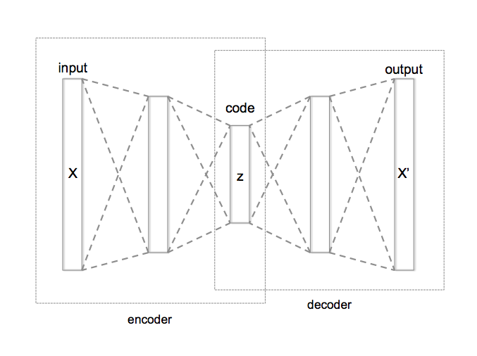
The index of the layer to use as input to the neural network for predict and predictPoint (zero counting). The default of 0 is the first layer (the original input layer), 1 is the first hidden layer, etc. This can be used to access different parts of a trained neural network such as the encoder or decoder of an autoencoder.

tapOut

The index of the layer to use as output of the neural network for predict and predictPoint (zero counting). The default of -1 is the last layer (the original output layer). This can be used to access different parts of a trained neural network such as the encoder or decoder of an autoencoder.