
Neural Network Training
An overview of how neural networks learn.
This article provides guidance on using the neural networks found in the FluCoMa toolkit including some intuition about how neural networks learn and some recommendations for training. For more detailed information on the MLP parameters visit MLP Parameters. FluCoMa contains two neural network objects, the MLPClassifier and MLPRegressor. “MLP” stand for multi-layer perceptron, which is a type of neural network. “Classifier” and “Regressor” refer to the task that each MLP can be trained to do.
Supervised Learning
Both the MLPClassifier and MLPRegressor are supervised learning algorithms meaning that they learn from input-output example pairs. The MLPClassifier can learn to predict output labels (in a LabelSet) from the labels’ paired input data points (in a DataSet). The MLPRegressor can learn to predict output data points from their paired input data points.
Supervised learning is contrasted with unsupervised learning which tries to find patterns in data that is not labeled or paired with other data. FluCoMa also has unsupervised learning algorithms such as PCA, KMeans, MDS, UMAP, and Grid.
The Training Process
Feed-Forward
The internal structure of a multi-layer perceptron (MLP) creates a “feedforward” network in which input values are received at input neurons, passed through sequential hidden layers of neurons which compute values that are passed on to the following layer, eventually arriving at output neurons which provide their values as the output of the neural network. These sequential layers are “fully connected”, meaning that each neuron in one layer connects to every neuron in the following layer. These connections are weights that are multiplied by the values to control how much each neuron’s output influences the neurons it is connected to. The neurons (except in the input layer) also use a bias (an added offset) and an activation function to compute its output. The weights and biases are internal parameters that are not controlled at all by the user.
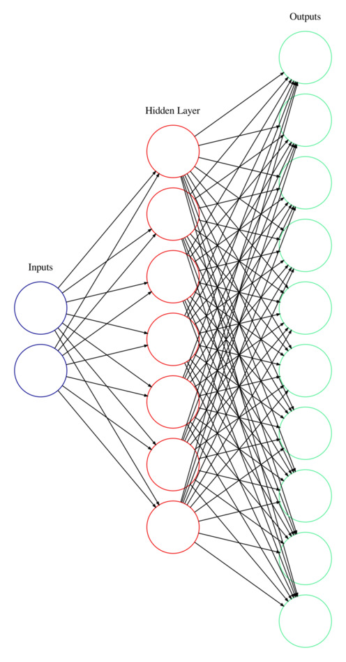
A multi-layer perceptron neural network that takes two inputs, has one hidden layer of seven neurons, and predicts ten outputs. Each black arrow is a weight. Each of the neurons in the hidden layer and output layer also have a bias.
Audio Mixer Metaphor
A useful metaphor for understanding how the feedforward algorithm works is to think of a neural network like an audio mixer. The inputs to the neural network are like the audio inputs to the mixer. The weights are like volume adjustments that control how much of an input signal gets passed on (in the case of a neural network, passed on to the next layer). The biases are like DC offsets that just shift the signal up or down. Activation functions are like distortion—they introduce some non-linearities into the signal (which for neural networks help them learn non-linear relationships between the inputs and outputs). Lastly, the outputs of the neural network are like the outputs of the audio mixer—a volume adjusted, DC offset, and distorted combination of all the inputs.
Training
The message that tells an MLP to train is fit. fit is synonymous with “train”. Its terminology is similar to “finding a line of best fit” or “fitting a curve to data”. fit takes two arguments: 1. the inputs to the neural network (a DataSet) and 2. the outputs we want the neural network to learn to predict (a LabelSet for the MLPClassifer, a DataSet for the MLPRegressor). In order for the the neural network will know which inputs to associate with which outputs, the input-output example pairs must have the same identifier in their respective (Label- or Data-) Set.
During the training process, an MLP neural network uses all the data points from the input DataSet and predicts output guesses (either a label for MLPClassifier or a data point for MLPRegressor). At first these guesses will be quite wrong because the MLP begins in a randomised state. After each of these output guesses it checks what the desired output is for the given input and measures how wrong the guess was. Based on how wrong it was, the neural network will then slightly adjust its internal weights and biases (using a process called backpropagation) so that it can be more accurate the next time it makes a prediction on this input. After training on each data point thousands of times, these small adjustments enable the neural network to (hopefully!) make accurate predictions on the data points in the DataSet, as well as on data points it has never seen before.
The Error
Because training the neural network is an iterative process, it is likely that you’ll send the fit message to the neural network many times. Each additional time it receives fit, it continues training, picking up from wherever it left off (the internal state of the neural network is not reset). Each time it concludes a fitting it will return a number called the error (also known as the loss). The error is a measure of how inaccurate the neural network still is at performing the task you’ve asked it to learn (so it may need more training!). Generally speaking, lower is better because it means there is less error, therefore the neural network is more accurately performing the task it is learning.
There isn’t any way to objectively reason about how low of an error is “low enough” (and “too low” might mean the neural network is overfitting). Instead, we can tell if the neural network is learning by watching how the error changes over multiple fittings. If the error is going down then we can tell that the neural network is learning from the data it is training on (which is good). At some point the error will start to level out or “plateau”, meaning that it is no longer decreasing. This is also called ”convergence”. At this point the neural network isn’t improving any more. It seems to have learned all it can from the data provided. It has “converged”. At this point it would be good to start using the neural network model to make predictions, or perhaps test it’s performance on some testing data.
Tweaking the MLP Parameters
As you are observing how the error changes over multiple fittings, it may be useful to change some of the neural network’s parameters between fittings to see if it can achieve a lower error, or change how the error is decreasing. See the parameter descriptions below for more information about why and how you might tweak each of them specifically.
Because the parameters hiddenLayers, activation, and outputActivation change the internal structure of the neural network, the internal state of the neural network is necessarily reset and any training that has been done will be lost. Even so, it is a good idea to play with these parameters because they can have a significant impact on how well and how quickly the neural network is able to learn from your data. All the other parameters can be changed without losing the internal state.
One strategy of training the neural network is to set maxIter rather low (between 10 and 50 maybe) and repeatedly call fit on the neural network. In Max or Pure Data, this might be using a [metro] (or [qmetro]). In SuperCollider this could be done by creating a function that recursively calls fit unless a flag is set to false (see the example code below). While these sequential fits are happening, watch how the error changes over time and adjust some of the MLP parameters as it is training to see how they affect the change and rate of change of the error value. Finding which parameters create a good training (convergence at a low error) is often a process of testing various combinations of parameters to see what works best. All of the parameters are worth experimenting with! And as always, make sure to test the performance of the neural network model to see if it really does what you hope!
s.boot;

// some audio files to classify
(
~tbone = Buffer.read(s,FluidFilesPath("Olencki-TenTromboneLongTones-M.wav"),27402,257199);
~oboe = Buffer.read(s,FluidFilesPath("Harker-DS-TenOboeMultiphonics-M.wav"),27402,257199);
)

// create a dataSet of pitch and pitch confidence analyses (and normalize them)
(
~dataSet = FluidDataSet(s);
~labelSet = FluidLabelSet(s);
~pitch_features = Buffer(s);
~point = Buffer(s);
[~tbone,~oboe].do{
	arg src, instr_id;
	FluidBufPitch.processBlocking(s,src,features:~pitch_features,windowSize:2048);
	252.do{ // I happen to know there are 252 frames in this buffer
		arg idx;
		var id = "slice-%".format((instr_id*252)+idx);
		var label = ["trombone","oboe"][instr_id];
		FluidBufFlatten.processBlocking(s,~pitch_features,idx,1,destination:~point);
		~dataSet.addPoint(id,~point);
		~labelSet.addLabel(id,label);
	};
};
FluidNormalize(s).fitTransform(~dataSet,~dataSet);
~dataSet.print;
~labelSet.print;
)

(
// take a look if you want: quite clear separation for the neural network to learn (blue will be trombone and orange will be oboe)
~dataSet.dump({
	arg datadict;
	~labelSet.dump({
		arg labeldict;
		defer{
			FluidPlotter(dict:datadict)
			.categories_(labeldict);

		};
	});
});
)

(
// make a neural network
~mlp = FluidMLPClassifier(s,[3],activation:FluidMLPClassifier.sigmoid,maxIter:20,learnRate:0.01,batchSize:1,validation:0.1);

// make a flag that can later be set to false
~continuous_training = true;

// a recursive function for training
~train = {
	~mlp.fit(~dataSet,~labelSet,{
		arg error;
		"the current error (aka. loss) is: %".format(error).postln;
		if(~continuous_training){~train.()}
	});
};

// start training
~train.();
)

// you can make adjustments while it's recursive calling itself:
~mlp.learnRate_(0.02);  // won't reset the neural network
~mlp.batchSize_(2);     // won't reset the neural network
~mlp.maxIter_(50);      // won't reset the neural network
~mlp.validation_(0.05); // won't reset the neural network
~mlp.momentum_(0.95);   // won't reset the neural network

~mlp.hiddenLayers_([2]);      // *will* reset the neural network
~mlp.activation_(FluidMLPClassifier.tanh); // *will* reset the neural network

// when the loss has decreased and then leveled out, stop the recursive training:
~continuous_training = false;
Comparing MLP and KNN
FluCoMa has another pair of objects that do classification and regression with supervised learning: the KNNClassifier and KNNRegressor. The KNN objects work quite differently from the MLP objects, each having their strengths and weaknesses. You can learn more about how KNNs work at their respective reference pages. The main differences to know are that:
- the flexibility of the MLP objects make them generally more capable of learning complex relationships between inputs and outputs,
- the MLP objects involve more parameters and will take much longer to
fit(aka. train) than the KNN objects, and - the KNN objects will likely take longer to make predictions than the MLP objects, depending on the size of the dataset (although they’re still quite quick!).