
Why Scale? Distance as Similarity
The affects of scaling on measures of similarity
When trying to determine how similar or different data points are (for example, two MFCC analyses with 13 values each) we often measure the “distance” between the points in their multidimensional space as a consideration of their “similarity” (in this case, “multidimensional” means the 13 MFCC dimensions). Points that are closer in multidimensional space are regarded as being more similar while points farther away are assumed to be more different. These distances are often computed as the euclidean distance between two points, however other measures of distance also exist.
For more information about scaling, see the reference of the respective scalers (Normalize, Standardize, and RobustScale) as well as the page Comparing Scalers.
The most common reason for scaling (probably using Normalize, Standardize, or RobustScale) is to transform a DataSet that has dimensions with very different ranges so all the of the dimensions are in a similar range. If dimensions with very different ranges are used to compute the distance between points, the distances computed would be more greatly influenced by the dimensions with greater ranges. If all dimensions should be considered equally when computing distance, it is important all the dimensions have similar ranges.
Many machine learning algorithms base their calculations and results on these distance measures (including PCA, UMAP, MDS, KMeans, KDTree, Grid, KNNRegressor, and KNNClassifier). Therefore it’s very important to be aware of what the ranges of the data’s dimensions are and what affects these ranges could have on the results.
For example, we are going to compute the similarity between sound slices that are represented by two attributes with very different ranges: spectral centroid in Hz and loudness in dB. The spectral centroids could have a range of about 10,000 Hz (maybe 2,000 Hz to 12,000 Hz), while the loudnesses might have a range of only about 100 dB (-100 dB to 0 dB). If we were to plot these spatially such that 1 Hz = 1 dB we’ll see what looks like a flat line: because the ranges are so different (two orders of magnitude), we’re really only able to see the differences in one of the dimensions.
By zooming in a bit we can see that the nearest neighbour of any given point is essentially based on the proximity in the dimension with a greater range: spectral centroid, whereas the comparison of loudness in dB has much less impact on how distant the various points are from each other—and little to no impact on which point is the nearest neighbour.
Plotting Sound Slices where 1 Hz = 1 dB
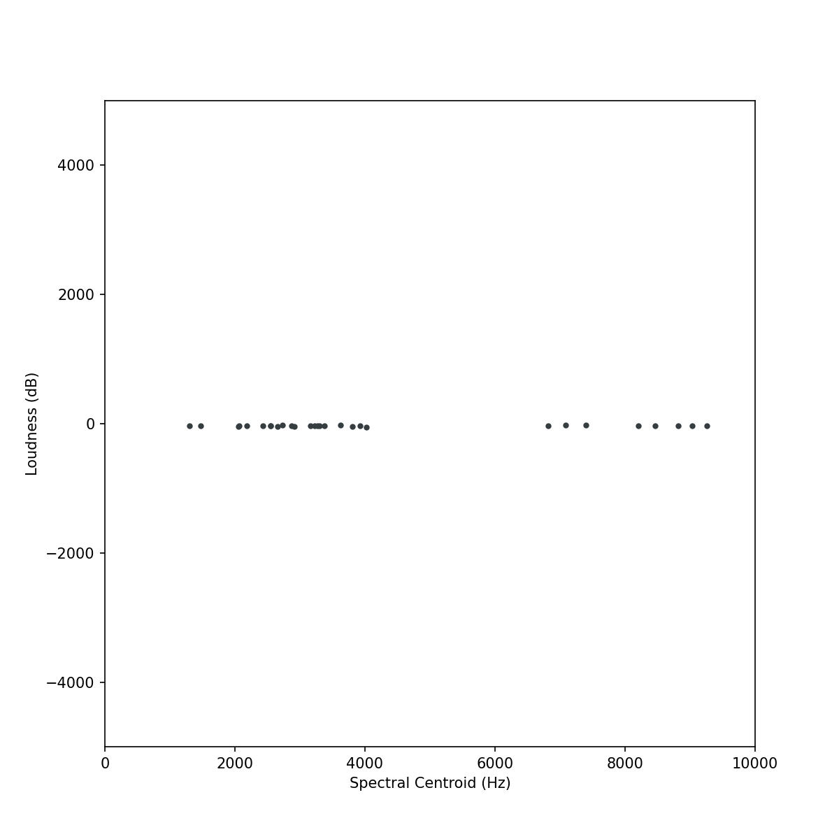
Sound slices plotted according to their spectral centroid and loudness on a plot where 1 Hz is spatially equal to 1 dB.
To consider this another way, imagine computing the distance between two points in a city (see the orange line below). To calculate the distance of the orange line, one would measure the east-west distance between the two avenues that the points are on (here shown as 100 dB or 100 not-to-scale city blocks) and the north-south distance between the two streets that the points are on (here shown as 10,000 Hz or 10,000 city blocks). The distance of the orange line can then be computed using the Pythagorean Theorem.
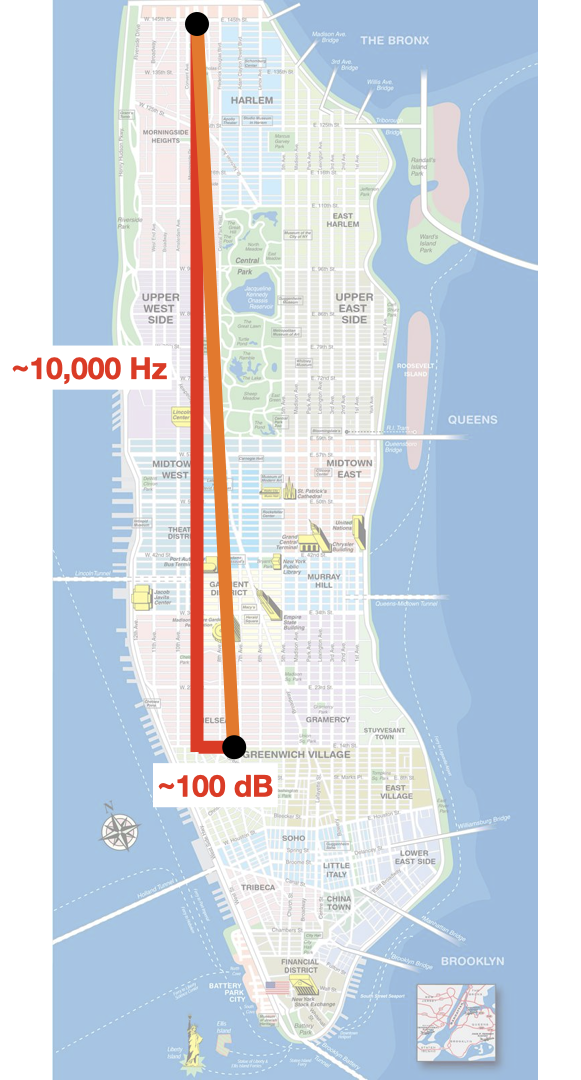
Finding the distance between two points using the Pythagorean Theorem where the two dimensions have greatly differing ranges.
Notice that the distance of the orange line is very similar to the distance of the vertical red line (~10,000 units). In fact, if the horizontal line (100 dB) were to double or halve in length, the distance of the orange line wouldn’t change very much. If the vertical red line were to double or halve in length, the orange line would change quite a lot! The distance of the orange line is much more influenced by the dimension that has a greater range (here, the vertical dimension).
Using a scaler (such as Normalize, Standardize, or RobustScale) can transform each dimension in a dataset into a more standard range (here used differently from the object Standardize), usually between 0 and 1 or centred around 0 with the other values as nearby positive and negative values. This scaling can ensure that all the dimensions used to compute distance are in a similar range and therefore will be equally influential in determining the distance between points.
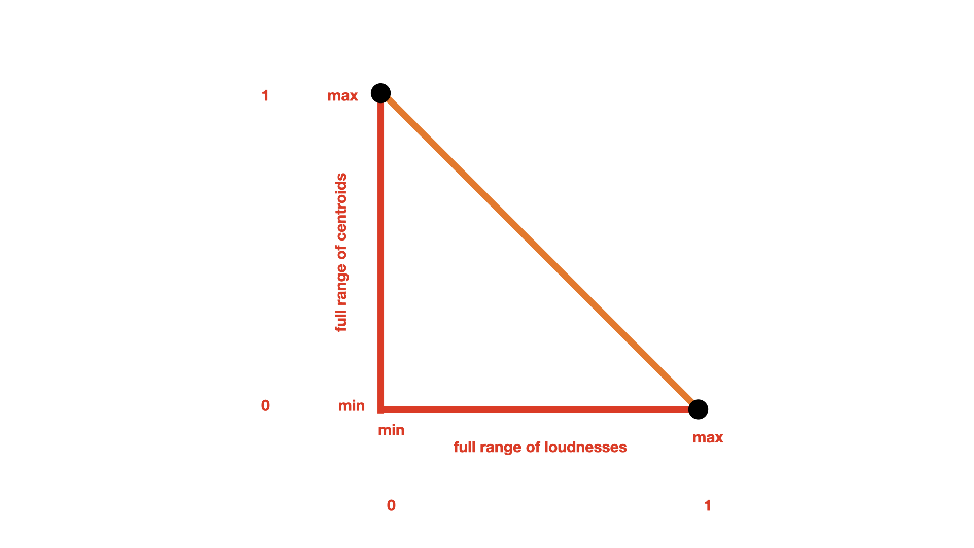
Finding the distance between two points using the Pythagorean Theorem where the two dimensions have been normalized between 0 and 1.
Linear vs Logarithmic Scales
Some audio analyses, namely pitch/frequency and amplitude/loudness, are commonly portrayed on a logarithmic scale instead of a linear one. Because logarithms distort ranges and scales (often in a useful way!), choosing one or the other will affect the distances calculated between points. It’s important to know which scale is being provided by an analysis and how it might affect your data. See the unit parameter in Pitch and SpectralShape for control over linear and logarithmic scaling.
For example, frequency analyses might be provided in hertz (which is on a linear scale), however this doesn’t reflect how humans actually perceive pitch distance. For a more perceptually relevant scale it is displayed logarithmically in pitch space (perhaps labeled as MIDI notes or semitones). If measuring in hertz, the distance from the A4 down one octave to A3 is 220 hertz, while the distance from A4 up one octave to A5 is 440 hertz—twice as far even though we perceive them to both be one octave! Measuring these distances in semitones however will reflect they way we perceive them: both a distance of 12.