
HPSS
Harmonic-percussive source separation using median filtering
Introduction
HPSS stands for Harmonic-Percussive Source Separation, which is designed to do what it sounds like: separate out the harmonic and percussive components of a sound.
This algorithm might be useful for general audio decomposition and remixing or for more specialised uses, such as extracting the harmonic component of a sound for use with a Pitch or Chroma analysis (which may improve their accuracy!) or extracting the percussive component of a sound for detecting onsets.
HPSS makes certain assumptions about what it is looking for in a sound: it is based on the observation that in a spectrogram “percussive” elements tend to form vertical “ridges” (tall in frequency band, narrow in time), while stable “harmonic” elements tend to form horizontal “ridges” (narrow in frequency band, long in time).
The spectrogram below shows 6 guitar strums. The “percussive” elements of this sound are the tall thin ridges at the attack of each strum (the percussive ridge of strum 3 is highlighted in pink). The harmonic element consists of the horizontal ridges which are the sustaining partials of the guitar strings (the harmonic ridges of strum 3 are highlighted orange).
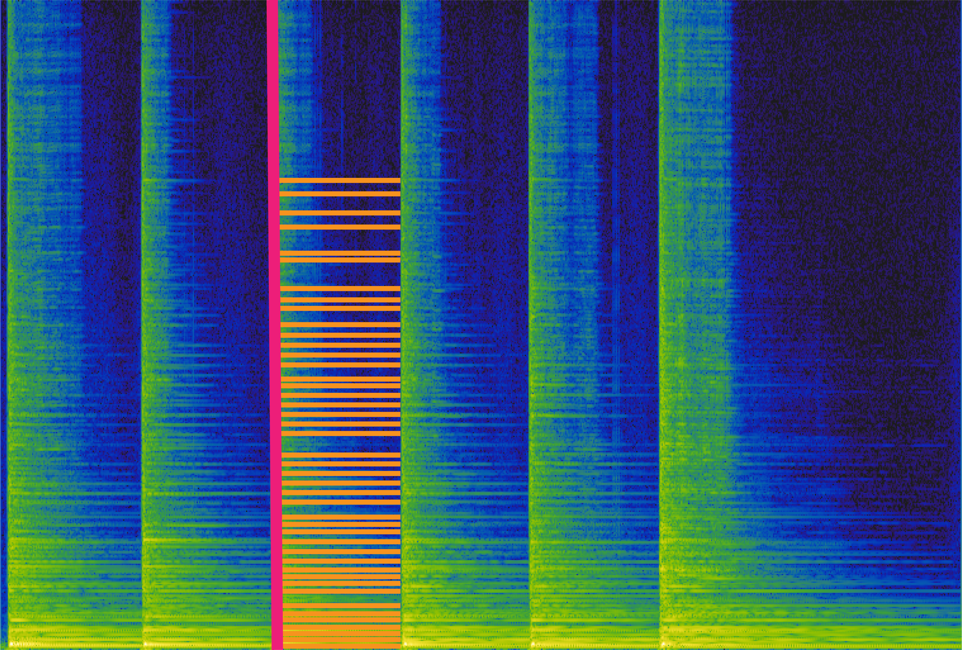
Spectrogram of guitar strums. Pink line shows a percussive moment ('vertical ridge'). Orange lines show harmonic content ('horizontal ridges') for strum #3
HPSS attempts to separate out each of these components by first creating a “harmonic-enhanced” spectrogram and a “percussive-enhanced” spectrogram.
Harmonic-Enhanced Spectrogram
HPSS creates the harmonic-enhanced spectrogram by running a median filter over each row of this spectrogram (one row here contains the magnitudes of a single FFT bin, or frequency range, over the all the frames of the spectrogram).
One row in this spectrogram represents a single frequency range over the entire duration of the spectrogram.
The plot below shows the magnitudes in that row (blue line) over the whole duration of the sound, revealing the six “percussive” strums that occur. The orange line shows the result of applying the median filter and how those “percussive” parts of this row are very suppressed. One can think of these percussive moments as outliers that are somewhat removed by the median filter. The larger that the argument harmFilterSize is, the more these “percussive” moments will be suppressed, and therefore removed from the harmonic-enhanced spectrogram.
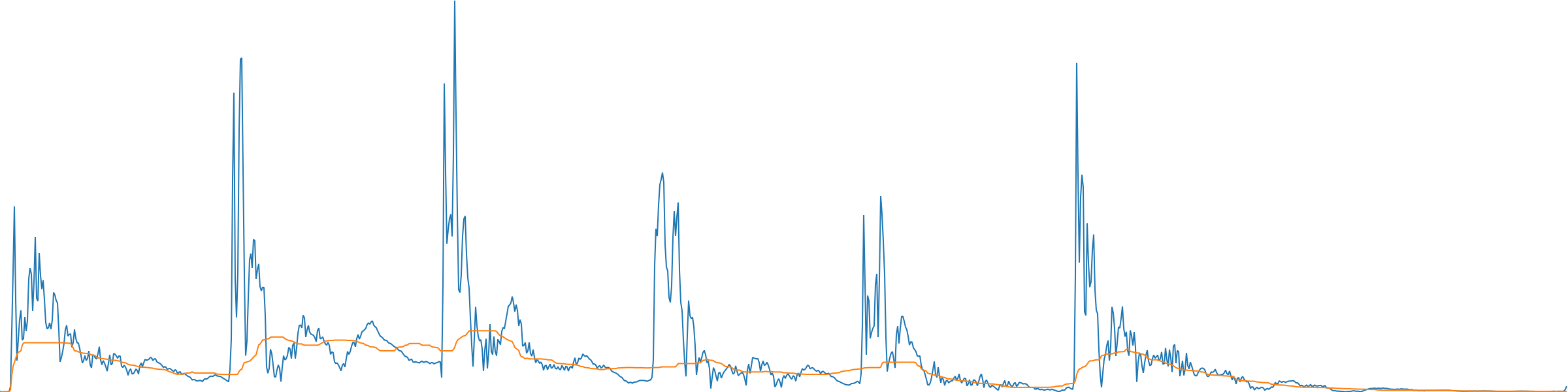
One row (FFT bin) of the spectrogram. x axis = time; y axis = magnitudes; median filter length = 51
After applying a median filter to all the rows, the resulting spectrogram is seen below.

Harmonic-Enhanced Spectrogram
Notice how the horizontal “harmonic” ridges are preserved, while the vertical “percussive” ridges are mostly removed. This is HPSS’s “harmonic-enhanced spectrogram”.
Percussive-Enhanced Spectrogram
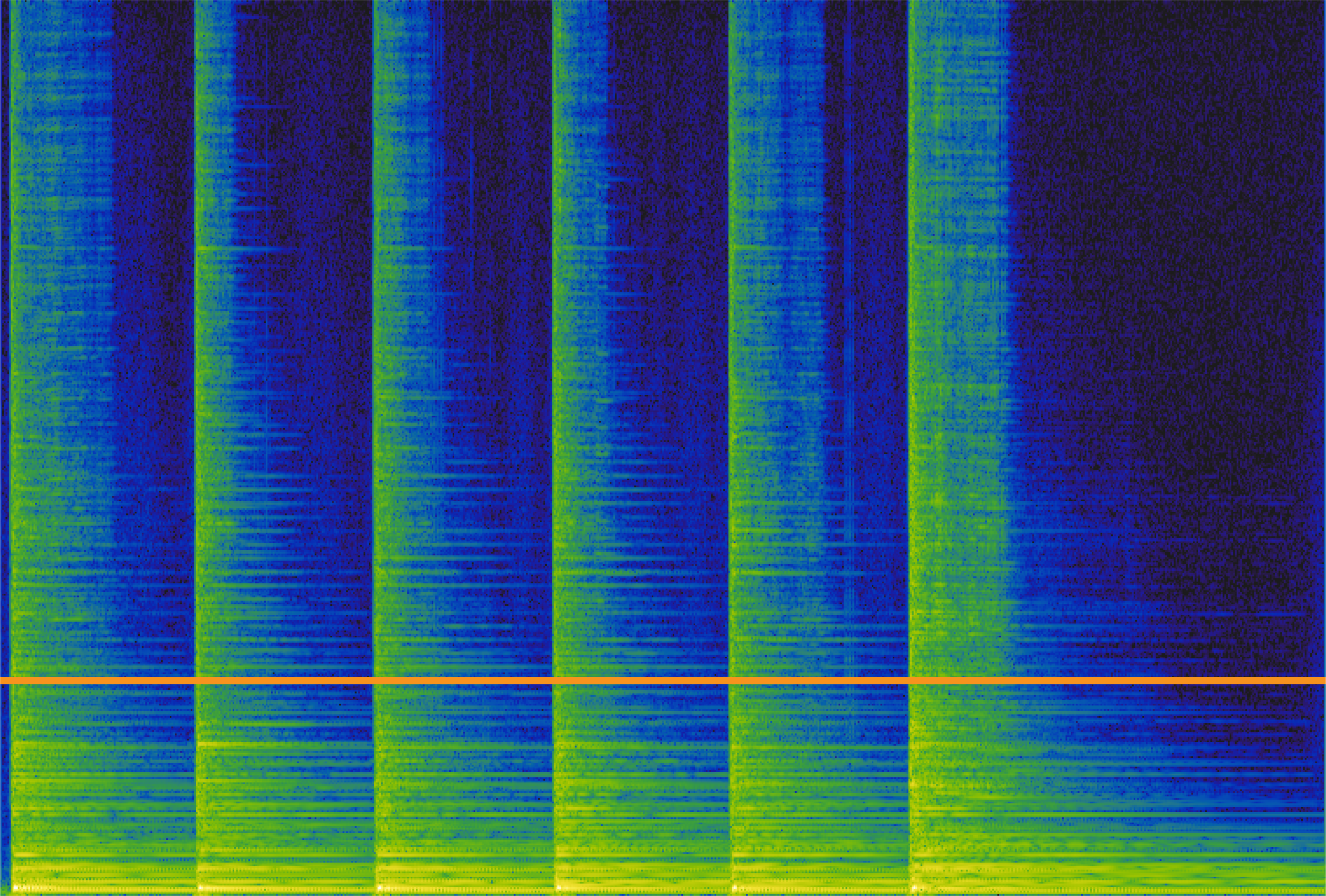
The percussive-enhanced spectrogram is created in a similar way. Instead of rows, the median filter is applied to each column in the spectrogram. The plot below of the original spectrum highlights one column. Below that is the magnitude spectrum of the highlighted frame (blue line).
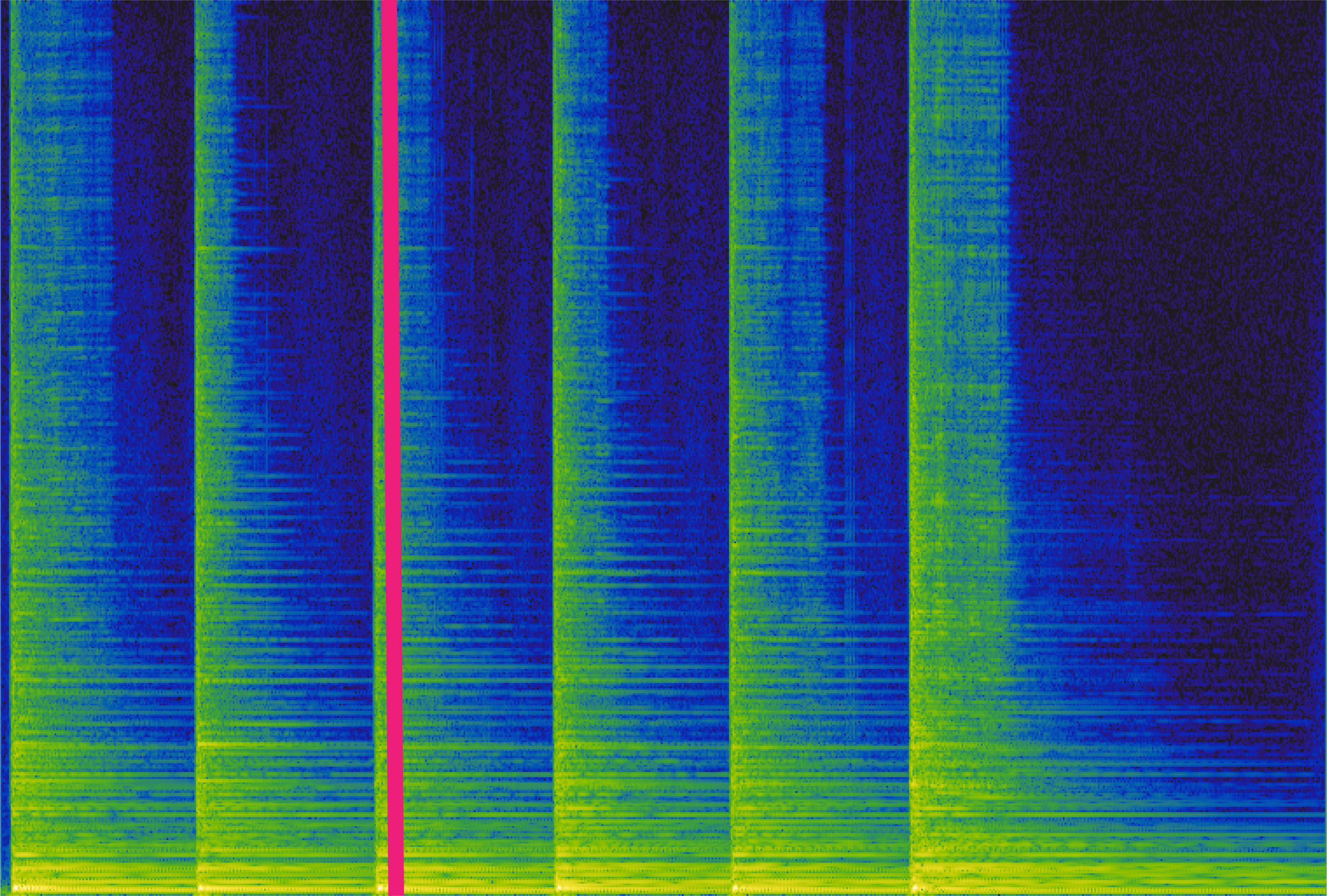
One column in this spectrogram represents a moment in time (one FFT frame).
One column (FFT frame) of the spectrogram. x axis = FFT bins; y axis = magnitude; median filter length = 91
The many peaks and valleys in this magnitude spectrum (blue line) are created by the harmonic structure of the sustaining guitar strings (i.e., the “harmonic” part of the sound). The orange line shows the result of applying a median filter to the magnitudes. You can see how the harmonic information in the spectrum is greatly suppressed. Again, the median filter removes what seem to be “outliers,” in this case harmonic peaks. The larger that the argument percFilterSize is, the more these harmonic peaks will be suppressed, and therefore not represented in the percussive-enhanced spectrogram.
Applying this median filter to all the columns creates the percussive-enhanced spectrogram seen below.
Percussive-Enhanced Spectrogram
Notice how the horizontal harmonic ridges are completely smoothed out: that information is no longer represented in this spectrogram. Instead what remains are strong clear vertical bars showing the percussive attacks of the guitar strums.
Masking
The next step is to create “masks”. Masks are the same shape as these spectrograms (same number of rows and columns) but instead of containing magnitudes they contain multipliers. These masks are created by comparing the harmonic-enhanced and percussive-enhanced spectrograms point-by-point and calculating what multiplier should go in the harmonic mask and what multiplier should go in the percussive mask. FluCoMa’s HPSS object has three options for how these masks are calculated.
After generating these masks (described in detail below), they are multiplied by the magnitudes in the original spectrogram to create the output percussive and harmonic components.
Binary Mask
The most basic kind of mask is the binary mask, which means it is filled with the binary options: zero or one. To use binary masking with FluCoMa’s HPSS object, the maskingMode argument must be set to 1. The harmonic and percussive binary masks are created by comparing each point in the harmonic-enhanced and percussive-enhanced spectrogram (each magnitude at each point in time) and simply seeing which is larger. If the magnitude in the harmonic-enhanced spectrogram is greater than the same one in the percussive-enhanced, then the harmonic mask gets a 1 at that point and the percussive mask gets a 0 and vice versa.
In the plots below you can see that the same spot is compared in each enhanced spectrogram (the red square, which is enhanced in size for clarity). Since the percussive-enhanced has a greater magnitude at that point (green is > than blue), the percussive binary mask gets a 1 (yellow), while the percussive gets a 0 (blue).

Comparing the same point in the harmonic- and percussive-enhanced spectrograms to create binary masks.
Notice how the harmonic and percussive binary masks are inverses of each other. Each point is the opposite of same point in the other mask. This means that when these masks (which are filled with zeros and ones) are multiplied by the original magnitudes to create the harmonic and percussive components, each magnitude in the original spectrogram will appear in only one of the two components. (In the “output” spectrogram plots below, black = a magnitude of zero.)
The output component spectrograms are created by multiplying (point-by-point) the original spectrogram with the component’s corresponding mask.
Harmonic Component Output Spectrogram (created using a Binary Mask)
.png)
Harmonic Component Output Spectrogram (created using a Binary Mask)
Notice how the horizontal harmonic ridges identified earlier are clearly present, including the rich lower partials of the guitar strums (the yellow ridges near the bottom). Also the vertical percussive ridges of the guitar strums are almost entirely black (a magnitude of zero), meaning they’ve been placed in the percussive output.
Percussive Component Output Spectrogram (using a Binary Mask)
.png)
Percussive Component Output Spectrogram (created using a Binary Mask)
Here we see the vertical percussive ridges of the guitar strums strongly represented. The lower partials of the harmonic guitar sustains (the yellow horizontal ridges above) are completely absent, as seen by all the black near the bottom. Although we do see some horizontal structure in this spectrogram, notice that it is filled with blue, meaning the magnitudes are rather quiet. These blue bands are the inverse of the much louder (yellow) horizontal ridges represented in the harmonic component output spectrogram above.
Output Audio
After creating the harmonic and percussive output spectrograms, FluCoMa’s HPSS object turns these back into separate audio streams as the final output of the object. The results when using binary masks (maskingMode = 1, heard directly below) tend to have stronger separation between the harmonic and percussive components, but also leave more sonic artefacts. The default (maskingMode = 0) uses soft masks (described later), which tends to leave much fewer sonic artefacts, but allows more bleed between the harmonic and percussive components.
More Masking Modes
Soft Mask
Rather than being filled with only zeros and ones like the binary mask, a soft mask can contain numbers between zero and one. These values are determined by the ratio between the two “enhanced” spectrograms so that each mask has a proportional amount of the energy. Like the binary masks, these soft masks are still inversely related. If one added them together all the points would equal 1, accounting for all of the energy in the original spectrogram. To use a soft mask with FluCoMa’s HPSS object, set maskingMode = 0, which is the default.
.png)
Harmonic Soft Mask
.png)
Percussive Soft Mask
.png)
Harmonic Component Output Spectrogram (created using a Soft Mask)
.png)
Percussive Component Output Spectrogram (created using a Soft Mask)