
Sines
Decomposition using a sinusoidal reconstruction model
Introduction
Sinusoidal modelling is probably the most venerable and widely researched STFT-based analysis and re-synthesis approach. It makes the strong assumption that a signal’s spectrum is dominated by a few well defined peaks, and that these vary slowly enough across time to be tracked as partials. For sounds that meet these assumptions, it can yield a much more compact representation with good results. The peaks can then be resynthesised either directly, using a bank of oscillators, or using an inverse STFT.
Some Practical Examples
Having taken an STFT, the first step is to estimate the peaks in each spectral frame (marked with red crosses below):
In practice, this is tricky, as a determination needs to be made about whether a peak in the spectrum represents a stable sinusoid, or is fleeting (and likely to be something noisier). Then, peaks need to be tracked from frame to frame to try and establish tracks of partials. Let’s breakdown the theory of this using some musical examples and spectrograms to help us. To start with, here is a spectrogram of a synth recording:
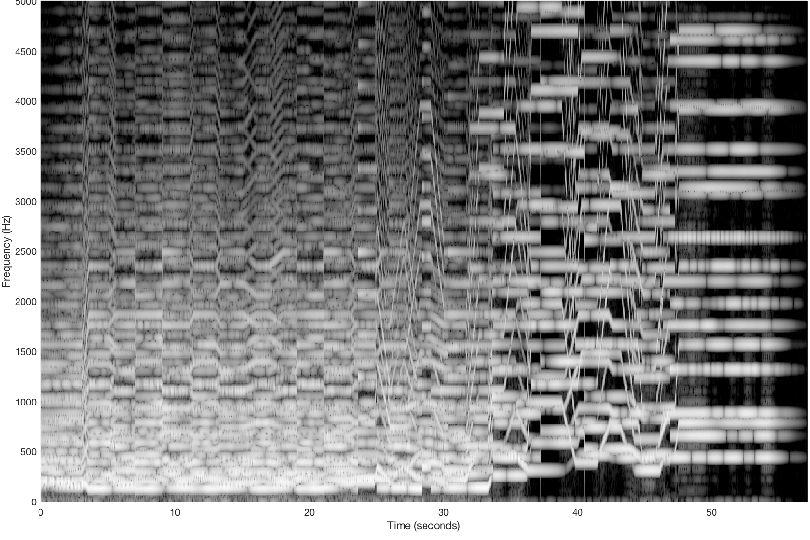
Spectrogram of a synth recording
The structure of partials should be pretty clear to see from the spectrogram. However, this is still giving the algorithm some work to do, because the partials in the sound cross each other at points. Here are some partial tracks overlaid on the spectrogram, and the resynthesised sound:
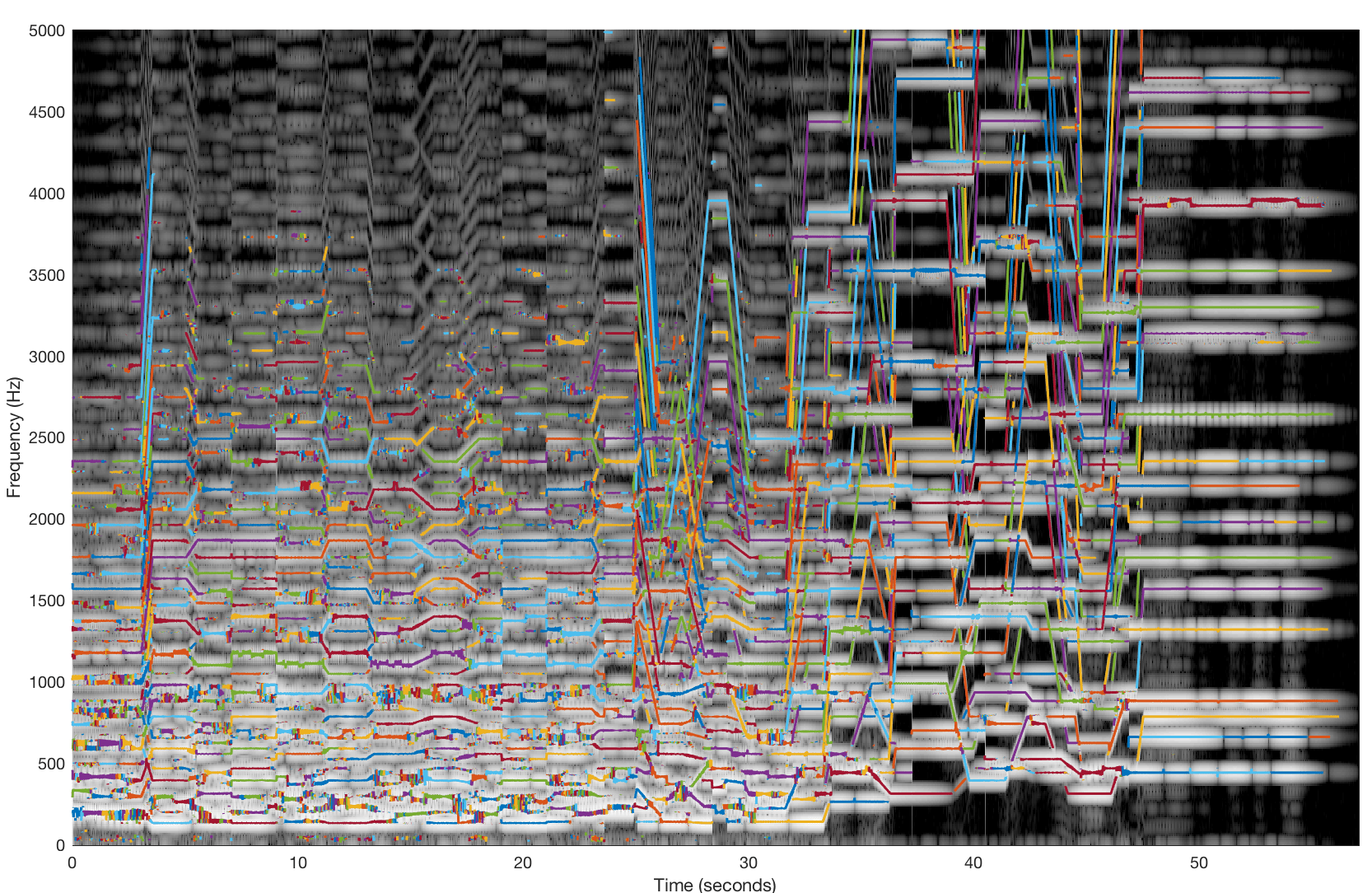
Spectrogram of the synth recording with partial tracks overlaid in colour
It didn’t do badly at all! Visually, it seems the algorithm gets a bit confused where partials cross each other in the spectrogram, and at higher frequencies (and note that we’re only getting up to about 5kHz). However, the resynthesis is pretty convincing. Ok, something harder. Let’s do a field recording:
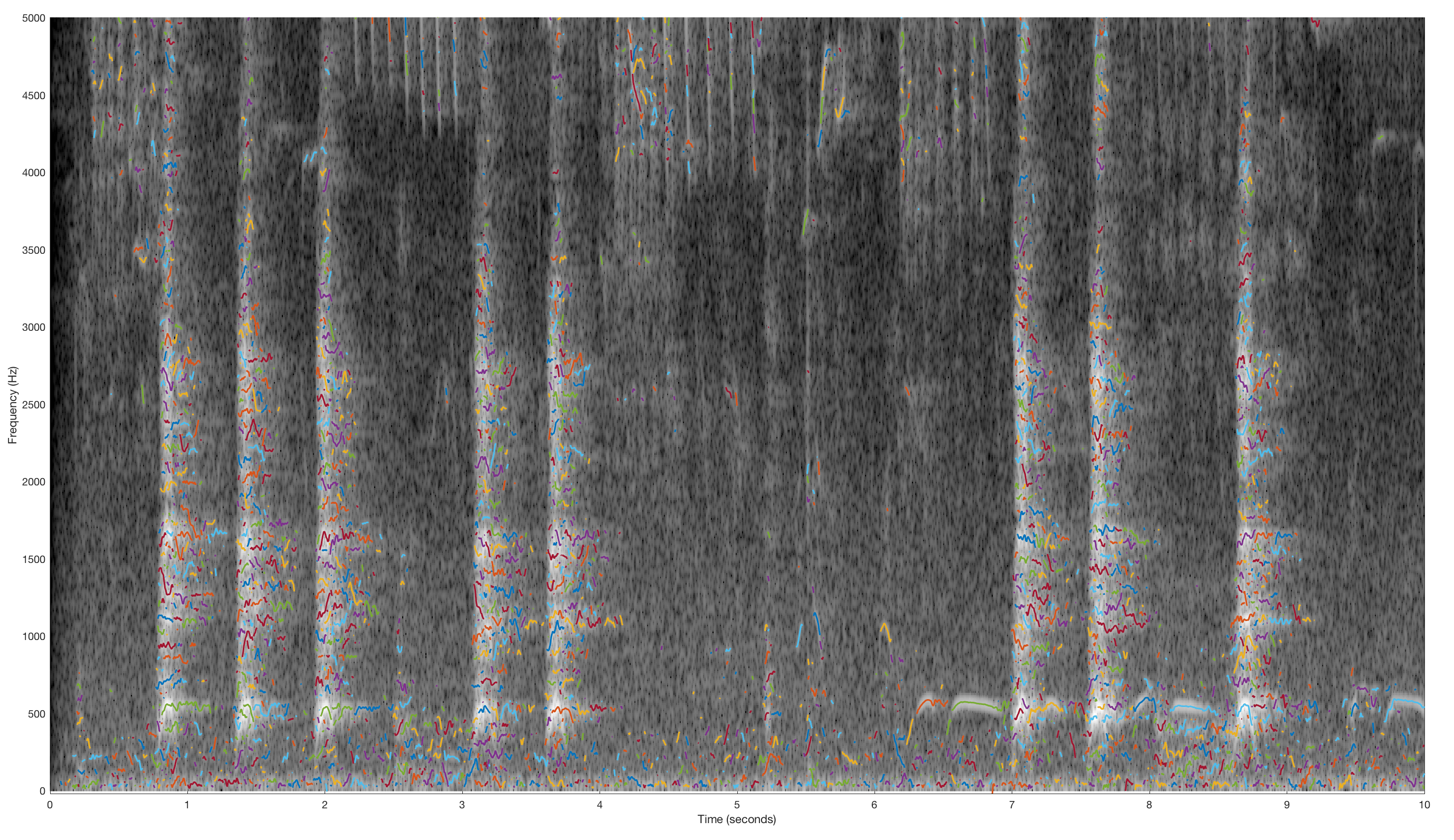
Spectrogram of a field recording with partial tracks overlaid in colour
Let’s compare the initial version with the resynthesised version:
We can both see and hear that this model struggles more here. The overall spectrum is denser, and has a less clear partial structure across time. We can see that it models the dog barks using a large number of brief sinusoid tracks, which shows that it struggles to model that component, and won’t be able to produce a compact representation of the signal. Whilst things sound ok at low volumes, we can hear how there is now a lot of low level “bubbly” interference, and the depth has gone from the sound. With that said, the parts that it has reproduced still sound like themselves. What we can do in the (frequent) case that sinusoidal modelling doesn’t model our sound well, is to take the residual (everything else) and use this as as a separate layer:
We could process it differently, or just use it to disguise the artefacts of the sinusoidal layer. Alternatively we could do further decomposition, for instance, to try and separate transients from noise. To explore that idea we might use some of the other objects from the FluCoMa toolbox such as Transients, HPSS or BufNMF.