
Filling the Shell
In this article we’ll be looking at the work Leafcutter John did for the project with his piece Line Crossing. We’ll take a detailed look at the workings of the piece, and how he used audio analysis to drive his bespoke audio modules.

Leafcutter John
Introduction
Download the demonstration patches for this article here.
Today we’ll be looking at the work John Burton (a.k.a. Leafcutter John) did for the project. A member of the first cohort of composers, he performed his piece Line Crossing at the first FluCoMa concert at HCMF 2019. The piece is fairly unique compared to others on the project: it is one of the only ones to have a specifically designed visual element as well as a sonic one. We shall be taking a dive into Burton’s musical and visual world, taking a detailed look at how this graphic score works and how he used some of the FluCoMa tools to drive some of its elements. As with all the ”Explore” articles, there is a series of demonstration patches that can be downloaded and interacted with if you wish to explore the inner workings of the software.
Burton performed Line Crossing at Bates Mill Blending Shed – of the five stages, his dominated the space from its central position and from the huge screen above it upon which the graphic score was projected. During the performance, his back was turned to the audience, however this did not separate him from us: everyone was turned towards the score that was emerging as the piece progressed. Burton plucked different instruments that were sat in a mess upon a table in front of him: cymbals, recorders, guitars, bows, sticks… Playing when the playhead entered the red blocks, his sounds were kept and recycled across the piece. The computer offers a polyphony of playback that spans from warm, pure harmonic tones that rub enticingly against each other; to chaotic cacophonies of crisp, percussive hits. Despite the stochastic nature of the piece and the improvised nature of the playing, there is still a positive sense of control over what is happening, and the sound emerges as being balanced with great skill.
There are three important parts that constitute this piece that we shall be looking at today: the graphic score and how it algorithmically creates itself; the audio processing and the way in which sound feeds back into itself through audio analysis with some of the FluCoMa tools; and the ways in which one can approach performance of this piece. Let’s begin by taking a look at the graphic score and how it drives the piece.
Graphic score
As you will have understood from the footage of the performance, the graphic score for Line Crossing has two main parts: a set of human blocks in red, and a set of “machine” blocks outlined in blue. These blocks can be of three different types: ramp up, ramp down and rectangular. We understand also from watching the performance what role the human blocks play: when the scrolling playhead is over one of the blocks, the performer makes some kind of sound. Finally, when the machine blocks are active, we understand that they seem to be playing back some of the audio played by the performer in some way.
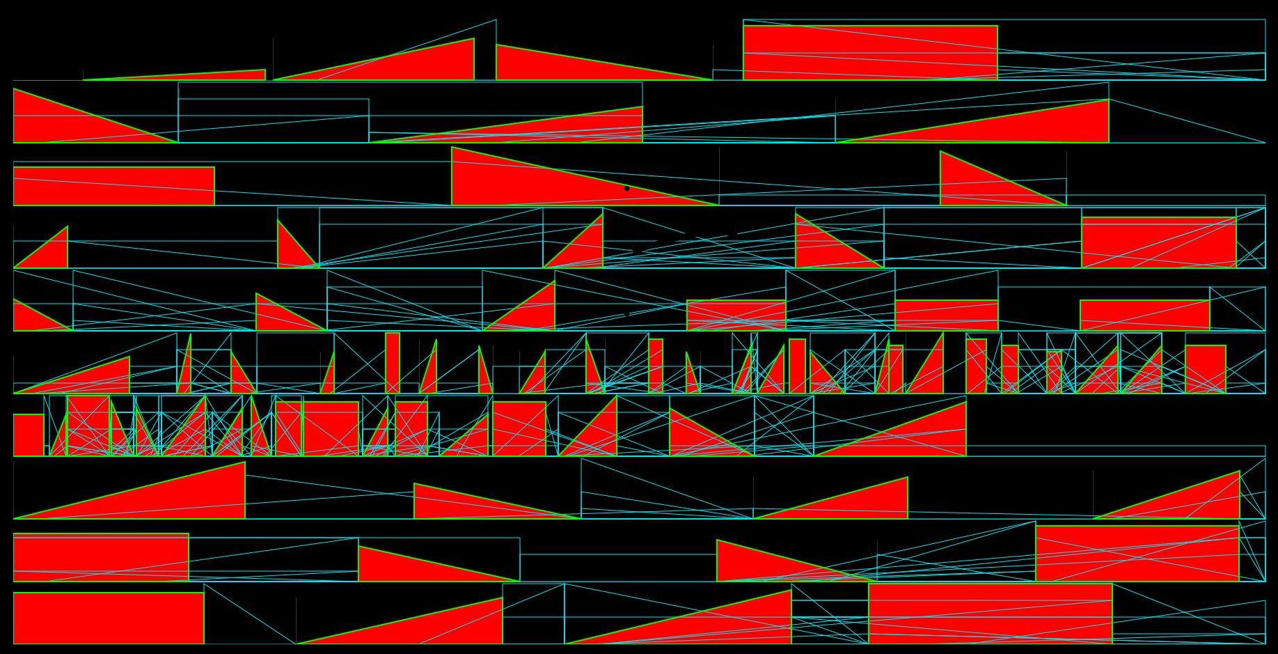
The score that was generated on the night of the performance.
There are also some other elements that are not apparent from merely watching the performance. We see that the score appears over the course of the performance – the score is always appearing at some point beyond the current playhead position; however, what we don’t know is that this score is being generated in real time stochastically. This means that Burton, the performer, knows where the score is going up to some point in the not-too-distant future, but that events are being generated algorithmically and there is no way of knowing precisely what will be generated ahead of time. The generation of the score is the first element that emerges from a stochastic, algorithmic process – the second is the configuration of and source sounds for the audio processing that we shall discuss in the next section.

The cover art for the album Yes! Come Parade with Us, made by Burton himself.
So how does this score work, and how does it fit in to some of Burton’s other works? What are the stochastic processes that are happening to create the score? Above, we see an image created by Burton for the cover of his 2019 album Yes! Come Parade with Us. He made this image by starting in the centre, and progressively drawing out the initial arc shape. As one can expect, there are moments where his hand may slip, or something may cause a slight imperfection to occur in the tracing of the initial shape. Over time, these slight blips get amplified, and they organically span out to create the final image that we see here. This is a process that appears to reoccur over much of Burton’s visual work. We shall discover that this kind of process resonates within the mechanics of this piece at several levels: not only in the stochastic creation of the score from a simple set of function objects, but also in the way analysis of the global output will inflect the processing of audio.
Another source of influence for the piece can be found in Stockhausen’s Elektronische Studie II (this patch is actually included in Max; go to Help -> Examples -> Synths -> Very Special Guest). Burton described Elektronische Studie II as “a more maths version [of Line Crossing] just with oscillators”. There are certainly flagrant similarities in aspects of the visual part of the piece, however Burton explained that his goal was to take this inspiration and make something that would respond to what he was doing, “to incorporate live sampling rather than just using oscillators”.
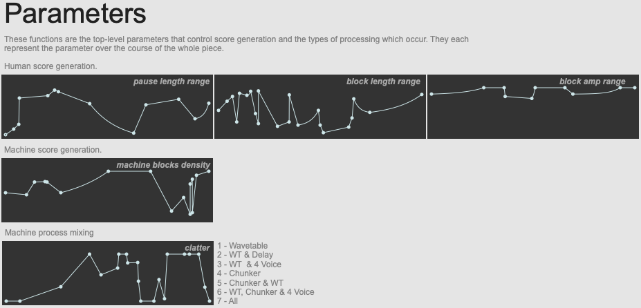
The top-level function objects used to generate the piece.
Burton started work on the piece with the score generation, and as development went on, he progressively introduced what turned into the function objects mentioned above which ultimately control the shape of the entire piece. As you can see, there are three objects which control aspects of the human score: pause length range, block length range, and block amplitude range. Notice that these objects are setting ranges and not specific values, meaning that there is still scope for randomness in the generation. That being said, we can see that there are definate correlations between the shapes that are seen here, and the score that was generated on the night: notably with the block pause length and length getting shorter towards the middle of the piece.
This is also reflected in the machine block density parameter, which is at its most dense towards the middle. As we shall see, there are 16 machine voices that can be running at any given time, and this controls to what extent these may all be triggered. Finally, there is a machine process mixing parameter that we shall return to in the next section. Burton described the main two parameters as being the pause length and human length of the blocks, explaining that they have the most agency over the shape of the score. He explained that the other parameters were implemented to “make the piece more playable”.
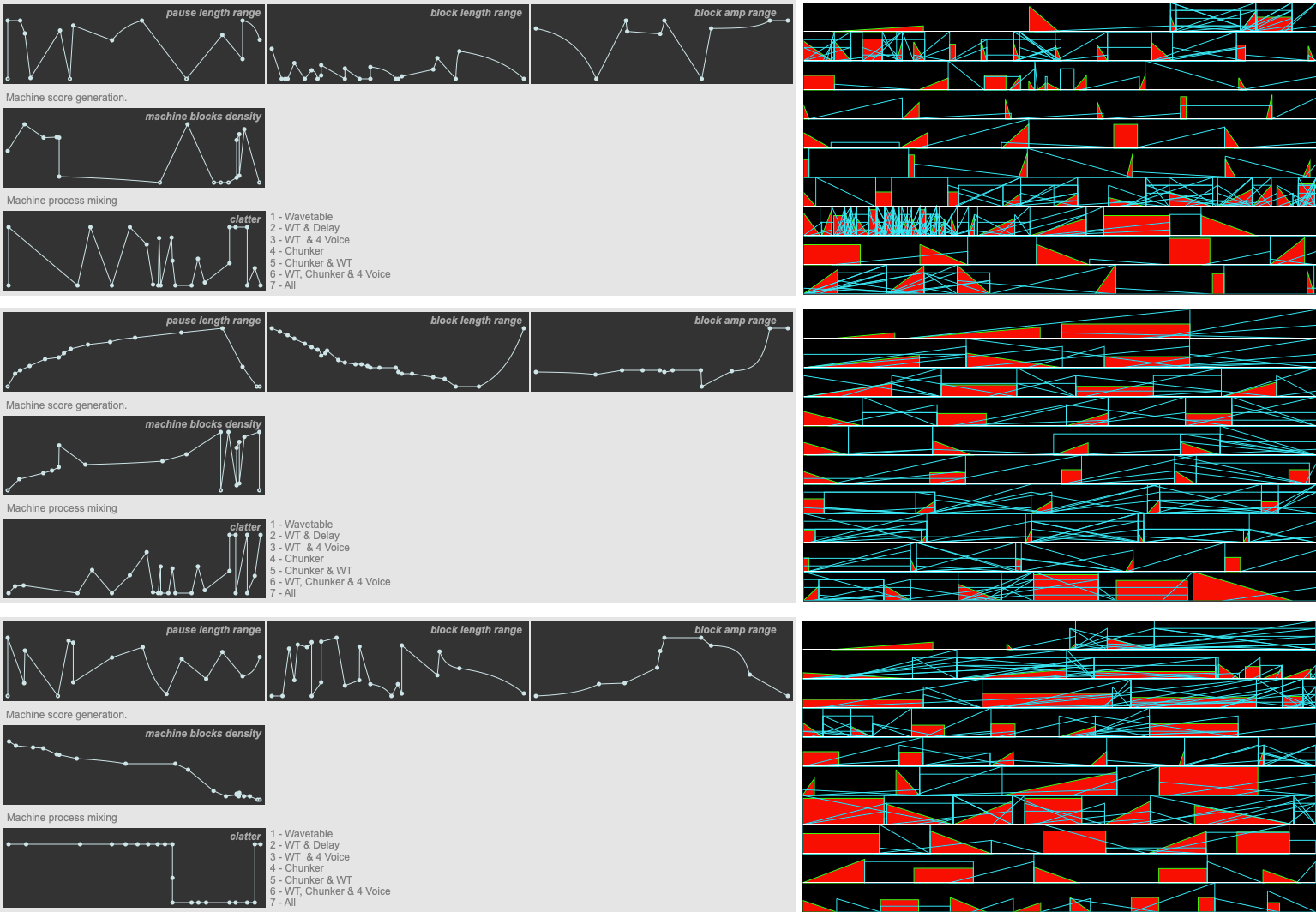
Different scores created with different parameters.
The score is constructed in Max with an lcd object. The length of the piece is actually tied to the ‘physical’ size of this object – advancing a pixel every 33ms. All of the onset times and lengths of the blocks are calculated according to this scale. In the example patches, the score you see is actually a recreation of this process using a JSUI object that can be resized: this makes it easier for analysis, but it’s interesting to bear in mind the original configuration that Burton dealt with during development, and how the ‘physical’ aspect of the score will have inflected his musicking.
The scores are stored in coll objects, which means that scores can easily be saved and recalled. At the beginning of the piece two human blocks are initially created to get the ball rolling. From then on, a new human block is created once playback reaches the end of a human block. Machine blocks are created whenever a new human block is created – the range of number of blocks created at a given point being controlled by the parameters set by the function object mentioned above.
This slightly-ahead-of-time way in which the score is created emerges then in part from the technical way Burton configured his patch. Burton also explained that this was necessary to be able to perform with it. He noted specifically that jumping lines is tricky – he explained that “you can judge speed when its moving across the page, but when it jumps it’s really hard to maintain that idea of when to play”. The way in which the score is generated tries to cater to this.
As mentioned above, this is where Burton began development of the piece. The visual aspect is very important – here and in other examples of his work. Progressively, Burton began to add audio processing that was informed by this somewhat pre-existing score. As reflected in the final nature of performing this piece, the score exists as a structure to be filled with sound, an abstract indication of form that could have been taken down various paths. Let’s now examine how Burton began to fill that shell.
Audio Processing
As mentioned above, there are 16 different voices that are triggered by the machine blocks. Each time a block is reached in playback, a free voice is found and will process audio in a number of different ways. You will recall from the piece parameters a function object that controls the machine processing mixing range. There are four different audio processing modules for each voice: wavetable, delay, chunker and 4 voice. The machine processing mixing controls the possible mix of these modules in the following way:
- 1: wavetable.
- 2: wavetable and delay.
- 3: wavetable and 4 voice.
- 4: chunker.
- 5: chunker and wavetable.
- 6: wavetable, chunker and 4 voice.
- 7: all.
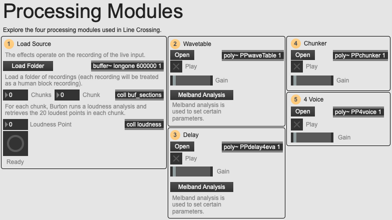
An overview of the 02 Processing Modules example patch.
We see that, the higher the control value, the more processes we will hear. This corresponds to the nature of the piece, with the much more chaotic and busy middle section. Remember that this control value is setting the top of a random range, meaning that if set to 7, there is still a chance that the machine block will only be set to wavetable. Let’s get to know these effects a little: if you open the example patch 02 Processing Modules you can experiment with the different modules separately and get to know how they sound.
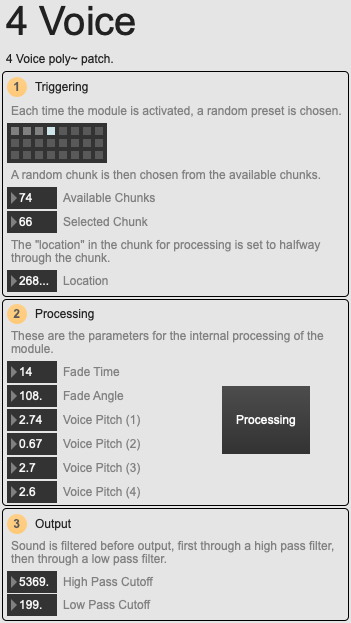
An overview of the 4 Voice module.
Burton explained that he wanted to “limit myself to tape techniques, playback at different speeds, because I actually like those sounds!”. This is most apparent in the 4 Voice module, which is incidentally the first module he made when he started getting “bored of doing the score with no sound”. Each time the module is activated, it will choose a random ‘chunk’ of recorded sound. A chunk corresponds to the recording of a human block: as the piece progresses, these all get recorded into a buffer along with the start and end times of the chunk. This means that as the piece progresses, more and more content will be available to the processing modules that use this audio. In the 4 voice module the chunk is taken and played-back through 8 separate groove~ objects which are looped until the module is deactivated. These are all playing at different speeds (voice pitch).

An overview of the Chunker module.
The three other modules begin to get a bit more complicated, but still retain the spirit of limiting the processes to tape techniques. First there is the Chunker module. When activated, an unstable pulse triggers playback of randomly selected chunks in four different streams. These are all enveloped slightly differently. The module has a characteristically percussive and rhythmic aspect.
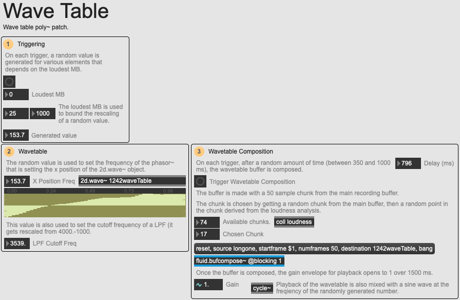
An overview of the Wavetable module.
In contrast with this there is the Wavetable module which delivers long, pure tones. It achieves this by choosing one of the recorded chunks, and composing a new buffer using fluid.bufcompose~ of 50 samples from the recording. The point in the buffer to be used is taken from a coll called loudness. This is where Burton’s use of audio analysis first comes into play: using fluid.bufloudness~, each time a human block is recorded, he takes the slice and retrieves the 20 loudest points within it. This is written to the loudness coll, meaning that each entry in the coll will correspond to a human block and its 20 loudest points.
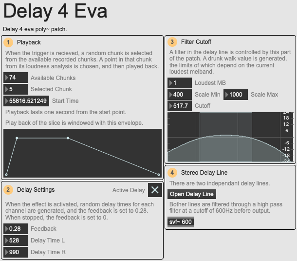
An overview of the Delay module.
This loudness analysis is also used in the final Delay module. When the module is activated, a random chunk and a random starting point from the loudness coll are chosen to begin playback. The audio is then played for 1 second, entering into a stereo delay line which can conceptually go on forever without fading away.
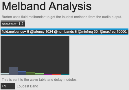
An overview of the melband analysis.
You will have also noticed that the wavetable and delay modules also derive some of their settings from another analysis: melbands. Burton is constantly performing two melbands analyses: one on the global output and one on the mic input. From this, he derives the loudest of 8 melbands, and sends this to the wavetable and delay modules. The delay module takes the band, and uses it to set the cutoff of a filter which has much agency over the aspect of the delay line. Essentially, the higher the loudest melbands, the lower the cutoff of the filter will be.
Similarly, the loudest melband is rescaled by the wavetable module in order to set the bounds of a random value which will be used to drive the frequency of the reading of the wavetable buffer, the cutoff frequency of a low pass filter and a low-pitched sine wave. Again, the higher the loudest melbands, the lower the generated values will be. It is interesting to examine the way in which Burton uses this audio analysis to progressively shape the general aspect of the piece. He is using it to control the various modules, and ensure that a certain balance in the spectrum is achieved. It is also interesting to consider that these changes will not be immediate: they will slowly evolve over time, subtly inflecting the output of the audio processing modules.
Again, it is best if you take a look at the modules yourself to hear what they really sound like. In the 02 Processing Modules example patch, you can load a folder of sounds, and each sound file will be treated as if it were a new recording in the human block buffer – you can even try this out with Burton’s own playing from the night, the recordings of which have been provided with the example patches. Now that we have an understanding of how the piece works, let’s take a look at how these elements come together to build a piece of music, and what it’s like to perform Line Crossing.
Performing
All these elements come together to make a unique structure within which one can perform. There are two recorded traces of performance: the first is the performance at HCMF, the second is when Burton gave a demonstration during his Traces of Fluid Decomposition presentation (see video below). You will notice that there are differences not only in the generated scores, but also in the ways in which Burton approaches performance: in the elements he plays and in the instrumentation.
Burton explained that the piece “could be played with anything, it doesn’t matter. You could do it in the hotel room hitting stuff, a load of people vocalising, you could even let it run on a train! It doesn’t make it more or less valid”. This throws up some interesting questions that were already underlined when looking at the development of the software: observing this approach, we really get the idea of the piece, the score, the patch and structure as an object to be filled with sound. This external structure is somewhat rigid, immutable (once it had been generated), and the soft, squidgy interior is more fluid, more living – biological matter that eases out like water to fill the hidden corners of the shell.
It’s interesting to consider this in regard to remarks that Burton made concerning the choice of the recorder as an instrument: “I’m not a trained recorder player, I can’t make beautiful notes, but that’s kind of why I chose that instrument. I’m definitely not interested in virtuosity in a traditional sense. There’s something I liked about the sort of wavery, pure tone of it. Blowing against the wavetables that the score was making – musically I liked it. It’s quite a warm tone against the cymbals.” This disinterest for virtuosity is interesting. This can suggest that the soft, sonic interior of the piece is not intended to be driven by rigorous, intellectually informed playing of an instrument - the word intellectual is used here in opposition to ideas of intuitive, affective appreciation and exploration of the sounds an instrument can make.
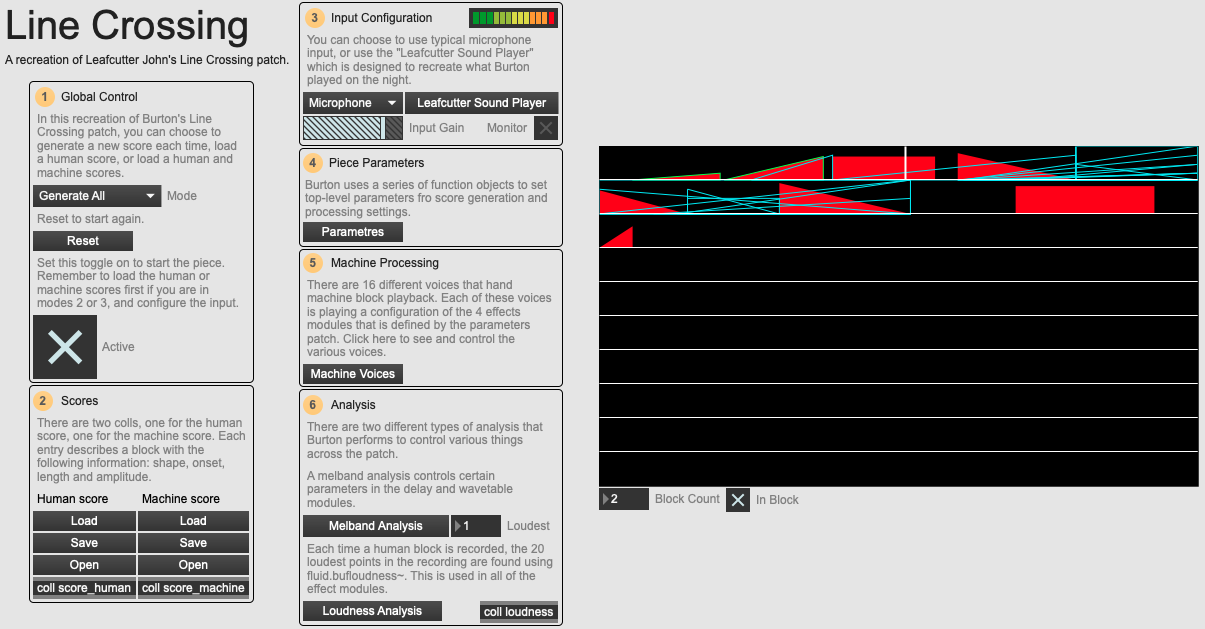
An overview of the 01 Line Crossing example patch.
The best way to understand what it can be like to perform with this system is to try it out yourself. With the example patch 01 Line Crossing you try things out with a number of different configurations. You can load the audio that Burton performed on the night and the machine and human scores to recreate that performance (still necessarily with stochastic machine processing choices). You can use this audio in a random order with newly generated scores to get something similar but different; or load your own audio or use the microphone to make your own performances!
Conclusion
Burton explained that “when you do a piece, [I feel like] you’re curating this sound world”. The software in Line Crossing reflects and extends this idea further than the choosing of sounds or instruments to include in a corpus. Here we see a system that invites the performer to build up a world progressively – a world of sound that will feed back into itself through analysis, that will grow and span out organically. Although very different in nature and in the way it’s played, there are many similarities to this in much of the software that Bruton produces. For example, take a look at a piece of software he has recently released, Forrester 2022. The user is asked to “build a forest”: a structure within which sounds are dropped, and a world is progressively built. This is a unique and inspiring way of making music and considering music software, which is so often presented as a stark tool, a grey means-to-an-end. Burton gives his software a certain spark of magic, personality and life which in turn will be heard in the music.