
Interface Design with FluCoMa
In this article, we take a look at some of the work that Sam Pluta did for the project. We look at his journey into exploring the possibilities of MLP regression, and how it has become an integral part of his practice.

Sam Pluta
Introduction
Download the demonstration patches for this article here.
In this article we will be looking at some of the work that Sam Pluta did for the project, and notably how he used MLP regression to augment his already well-developed SuperCollider modular system. We shall start by taking a look at his piece, a duo with trumpetist Peter Evans (in two parts: Neural Duo I and II) and an overview of Pluta’s instrument. Then we shall explore some of Pluta’s thoughts on MLP regression and his approach to training; before finally discussing some wider ideas around instrument design. As with all the ”Explore” articles, there is a series of demonstration patches that can be downloaded and interacted with if you wish to explore the inner workings of the software.
Due to travel restrictions at the time, both parts of the performance were pre-recorded and projected on the night of the second FluCoMa performance at Dialogues Festival 2021. The videos are edited in a way that give us a good view on what was happening: we have close-up angles of both Pluta and his various controllers (joystick, 2 iPads and a laptop) and Evans and his trumpet. The pair have been long-time collaborators, meaning that this was far from their first performance together. However, as we shall discuss below, in addition to pre-recording the performance, the pandemic also imposed another aspect on the performance which made it particularly unique for them.
The two performances are a fascinating counterpoint between the harsh digital noises of Pluta’s system and the wide spectrum of extended techniques performed on Evans’ traditional instrument. The two parts are different in nature: with the first, we are thrown straight into the action – the audience is immediately pulled along by an enthralling intensity of activity from beginning to end. The second eases us into a delicate and curious world of sounds that build into an enchanting dialogue between the two musicians. Through the two pieces, we understand that these two performers, and two instruments, propose a scope of sounds far beyond what we may expect.
It is clear the much work and experience has gone into the exploration of the sonic possibilities of these instruments. This is especially noteworthy with Pluta who not only plays his instrument but is the person that made it. It is the fruit of a career-long iterative development process, and over this time, Pluta has refined his approach to the art that is instrument-making. Indeed, he stated that for him, “the piece is really the software, the piece is this instrument which is now part of my setup. That, to me, is what was commissioned, not necessarily the performance that we saw.” Today we shall take a look at this artistic process by discussing how Pluta developed parts of his instruments with some of the FluCoMa tools and some of his broader ideas on HCI and instrument design. First, let’s get a better idea of how the piece and his instrument broadly work.
How it Works
The piece
With projects such as the Peter Evans Ensemble, Pluta and Evans have been working together for almost 15 years; but Pluta explained that this project represented a change in direction for them. In the past, much of Pluta’s practice involved live processing of the musician(s) with which he was playing. Here, Pluta isn’t doing any processing at all on Evans’ playing – he is simultaneously creating sound with a collection of synthesizers (see below) and processing their output. Pluta explained that this was a symptom of some of the circumstances that we all found ourselves in during lockdown: “I literally spent […] 16 months in my bedroom making music alone, so I developed a personal solo language that I didn’t actually have before”.
In addition to this, the pandemic imposed another logistical parameter on the piece: the two musicians recorded their parts separately. This is not something that they had done together before, and Pluta commented that it was quite an interesting experience. Pluta recorded an improvisation for Part I and sent it to Evan to play on top of, and the opposite happened for Part II. As we can hear, for Part I Pluta described going for an “all out, 7-minute noise-fest”. Evans said that this was quite challenging to play with – and the best strategy he found was to go with one idea and stick with it. Pluta described the part that Evans sent for Part II as “different, disjunct objects – some of which are very tonal”. To answer this, he tried to play “an accompanist role, but a weird accompanist who’s almost trying to make a contrapuntal music that isn’t necessarily connected”.
There are a few interesting elements to note about this configuration: first, Evans didn’t have a good idea about what Pluta was going to do with his track. Indeed, Pluta usually performs live processing on his collaborators, therefore this could explain the more disjunct, spaced-out nature of some of Evans’ playing. Pluta commented that Part II was “really weird in a way because of that”. In any case, Pluta purposefully chose this stem from a collection of others that Evans proposed for the very reason that it was so far removed from what he had imagined, and because it pushed him to play differently and learn some new ideas.
Another point to note is the inflected nature of the improvisatory practice that is occurring. This is not like a traditional live improvisation setting – Pluta explained that here, there’s an element of planning that you can do. You can “know ahead of time that the person’s going to change, so you can plan a change”. This undoubtedly influenced their performances compared to a live setting. The resulting pieces are certainly intriguing. Reflecting on them, Pluta said that “[the second one] definitely feels like we’re in separate rooms, but I like that. The first one almost feels like we’re in the same room and it’s kind of freaky in a way!”.
The Instrument
As mentioned above, Pluta’s modular SuperCollider instrument is a large focus of his artistic practice and has been for many years. He has written extensively about it, and also presented how it works in many contexts (see below). Today we’ll be focusing on some of the parts that make use of the FluCoMa toolkit, however we will give a broad overview of its configuration.
The software works conceptually very much like a modular synthesizer setup: there are various modules with inputs and outputs that can be fed into each other. The modular approach also means that it makes it very easy for Pluta to add to the system over time, having a somewhat agnostic framework that allows for new modules. Where Pluta’s system becomes particularly powerful, is the possibility to have multiple simultaneous banks of modular configurations. Pluta can define any number of configurations, and switch between them fluidly during performance. This grants an incredible versatility to his instrument. He explains in his PhD thesis: “by creating a setup where the performer is able to easily switch between combinations of sound modules, we create a system where multiple ways of interacting with sound are available to the performer at all times”.
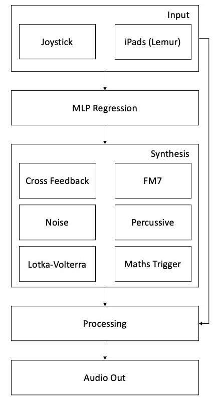
An overview of Pluta's instrument.
As explained above, the particularity for this piece is that Pluta is not processing the sound from the trumpet – only sounds from a set of synthesizers that he is controlling as part of his instrument. These are listed in the diagram above – he also explains some of them in this paper for AIMC 2021 which we shall return to below. In this diagram we see that Pluta is using an MLP regressor to map input from his to controllers: the joystick and the iPad (running Lemur). Due to the multi-configuration nature of the instrument discussed above, and to the way that the synthesizers are mapped, Pluta can actually be running up to 64 different instances of the fluid.mlpregressor object at any given time (he also uses fluid.dataset for interaction with these objects). Let’s now take a more detailed look at how these regressors are working for Pluta, and how he approached their training.
MLP & Training Process
Living in the NN Age
MLP regression is something that has been discussed previously in some of the FluCoMa “Explore” articles. You can learn about how it was used by Alice Eldridge and Chris Kiefer for their shared instrument here, and how classification was used by Alex Harker to explore oboe multiphonics here. The premise for using a neural network and regression in a musical context is fairly simple: taking an input of a certain number of dimensions and mapping it to an output of a different number of dimensions. This can be useful, for example, for controlling a synthesizer that has a high number of dimensions with a 2-4 dimensional input. This is the kind of process that Pluta explored. For those who are interested, there is also an in-depth FluCoMa tutorial on this subject.
In the AIMC paper discussed above, Pluta explains that synthesizers such as his Cross Feedback Synth and his DX7 emulation are perfect candidates to be controlled by neural networks, because there is “basically no other way to control those kinds of systems”. The cross feedback synth is extremely chaotic, and the slightest change of one parameter can drastically change the sound. Pluta described the DX7 emulation as being very “soupy and slow”, with over 50 control dimensions. They are both instruments that have a huge scope of sonorous potential. When experimenting, it can take a long time to find a new sound in the infinitely large range of possibilities – and in a live setting it becomes impossible to control them in a fluid manner. If you wish to experience this kind of synth for yourself, you can test the emulation of Pluta’s cross feedback synth provided in the example code for SuperCollider code given below.
//-----------------------------------------------------------------------------
// Cross Feedback Synth
//-----------------------------------------------------------------------------

// This is a recreation of Sam Pluta's Cross Feedback Synth from his
// live modular performances system:
// https://github.com/spluta/LiveModularInstrument

(
s.waitForBoot{

	//-------------------------------------------------------------------------
	// Data
	//-------------------------------------------------------------------------

	// Buffer for storing control data:
	~y_buf = Buffer.alloc(s,16);

	//-------------------------------------------------------------------------
	// GUI
	//-------------------------------------------------------------------------

	Window.closeAll;
	~win = Window("Cross Feedback Synth",Rect(0,0,600,400));

	// Output slider:
	~multisliderview = MultiSliderView(~win,Rect(0,0,400,400))
	.size_(16)
	.elasticMode_(true)
	.action_({
		arg msv;
		~y_buf.setn(0,msv.value);
	});

	// Add randomize button:
	Button(~win,Rect(400,0,200,20))
	.states_([["Randomize"]])
	.action_({
		arg but;
		var rand_values = ({ 1.0.rand } ! 16);
		~y_buf.setn(0,rand_values);
		~multisliderview.value = rand_values;
	});

	~win.front;

	//-------------------------------------------------------------------------
	// Synthesis
	//-------------------------------------------------------------------------

	~synth = {
		// Setting variables and retrieving control data:
		var localIn, noise1, osc1, osc1a, osc1b, osc2, out, foldNum, dust, trigEnv, filtMod, envs, onOffSwitch;
		var mlpVals = FluidBufToKr.kr(~y_buf);

		// Setting parameters from control data:
		var freq1 = Lag.kr(mlpVals[0], 0.05).linexp(0,1,2,10000);
		var freq2 = Lag.kr(mlpVals[1], 0.05).linexp(0,1, 5, 10000);
		var modVol1 = mlpVals[2].linlin(0, 1, 0, 3000);
		var modVol2 = mlpVals[3].linlin(0, 1, 0, 3000);
		var noiseVol = mlpVals[4].linlin(0, 1, 0, 3000);
		var impulse = mlpVals[5].linexp(0,1, 100, 20000);
		var filterFreq = Lag.kr(mlpVals[6], 0.05).linexp(0, 1, 200, 10000);
		var rq = Lag.kr(mlpVals[7],  0.05).linlin(0, 1, 0.2, 2);
		var fold = mlpVals[8].linlin(0,1,0.1,1);
		var dustRate = mlpVals[9].linlin(0,1, 1000, 1);
		var attack = mlpVals[10].linexp(0, 1, 0.001, 0.01);
		var release = mlpVals[11].linexp(0, 1, 0.001, 0.01);
		var outFilterFreq = Lag.kr(mlpVals[12],  0.05).linexp(0, 1, 20, 20000);
		var outFilterRQ = mlpVals[13].linexp(0, 1, 0.1, 1);
		var filtModFreq = mlpVals[14].linlin(0, 1, 0, 30);
		var filtModAmp = mlpVals[15].lincurve(0, 1, 0, 1, 1);

		// Synthesis:
		localIn = LocalIn.ar(1);

		noise1 = RLPF.ar(Latch.ar(WhiteNoise.ar(noiseVol), Impulse.ar(impulse)), filterFreq, rq);

		osc1 = SinOscFB.ar(freq1+(localIn*modVol1)+noise1, freq1.linlin(100, 300, 2, 0.0));
		osc1 = SelectX.ar(freq1, [osc1.linlin(-1.0,1.0, 0.0, 1.0), osc1]);
		osc2 = LFTri.ar(freq2+(osc1*modVol2));
		osc2 = LeakDC.ar(osc2);

		LocalOut.ar(osc2);

		out = [osc2.fold2(fold), osc2.fold2(fold*0.99)]/fold;
		dust = LagUD.ar(Trig1.ar(Dust.ar(dustRate), attack + release), attack, release);

		out = SelectX.ar((dustRate<800), [out, out*dust]);

		outFilterFreq = (LFTri.ar(filtModFreq)*filtModAmp).linexp(-1.0, 1.0, (outFilterFreq/2).clip(40, 18000), (outFilterFreq*2).clip(40, 18000));
		out = RLPF.ar(out, outFilterFreq, outFilterRQ);
		out = LeakDC.ar(out);

		Out.ar(0,LeakDC.ar(out,mul: 0.1));
	}.play;
}
)
As one experiences when experimenting with the synthesizer, it is a difficult instrument to handle. We can understand why Pluta looked to neural network technology in order to approach the controlling of this kind of instrument. Pluta described what it was like being a part of the FluCoMa community and being at the forefront of using this technology in an artistic context. He explained that we were at a “nascent stage with this technology [and that it is] both exciting and frustrating”. He compared it to reading Curtis Roads’ writing on granular synthesis: nowadays it seems elementary, but at the time it was very fresh. He explained that this is the first time in his career as an electronic musician that this has happened, and that it is extremely motivating. This also means, however, that he’s never failed as much in his life than in the 3 or 4 years working with these tools in the project!
One of these failed (but not abandoned) experiments was the idea to ring-modulate the real-time centroid and pitch analysis of the incoming trumpet signal with the x and y data of an xy pad to control a neural network. One of the main setbacks for this was issues with latency. Indeed, latency is a question that is dealt with by all creative coders who operate in the real-time, live domain. There are various examples of this across the “Explore” articles – for example the articles on Lauren Sarah Hayes’ work or Rodrigo Constanzo’s work.
Another experiment was a 2-dimensional space into which Pluta projected the PCA dimensionality-reduction of MFCC analysis data of a 3000-sample dataset, explained in the video above. Check out this FluCoMa tutorial on building your own 2D corpus explorer. He would navigate this digital space with his joystick, using the fluid.kdtree~ object to retrieve the nearest neighbours and play back the samples. In the end, he didn’t persue this avenue, notably because he much prefers to use synthesis than samples. However, parts of this can help us to understand his approach to instrument making, and to training the neural network.
Pluta has described two parts of the development process:
- Developing the synth.
- The curation of sounds from that synth.
In the video above, he explains that the idea was more or less to create as many (and varied) sounds as possible. This is reflected in the nature of the synthesizers that he develops to use with the neural networks: the cross feedback synth, the DX7 emulation, the Lotka-Volterra chaotic oscillator – these are all instruments that offer not only a slippery control space, but also a wide breadth of sonorous potentialities. Pluta describes these landscapes of infinite sonic variation as having these “little pockets of glorious sonic change and then vast wastelands of nothing”. He also explained the MLP’s role in this landscape: “training the neural network involves finding one of these pockets and training the network to exist within it”. Let’s look at this training process in more detail.
Approach to Training
Pluta will iteratively build up a corpus of mappings, iteratively build up his instrument. We have built an example environment in SuperCollider using the cross feedback synth that should allow you to experiment with this same kind of process. This can be done with a digital control surface; however, we suggest finding a physical HID – even if it’s just a mouse! We shall discuss how Pluta approaches the selection of his HIDs in the next section.
//-----------------------------------------------------------------------------
// Corpus of Mappings
//-----------------------------------------------------------------------------

// This is based on the "Neural Network Controls Synth from 2D Space" example,
// found in the FluCoMa Examples folder. For a more detailed description about
// what is happening, please consult that example.

// Here, we have created an environment which allows the user to build up a
// "corpus of mappings" between a 2-dimensional pad and the 16 control
// dimensions of Pluta's "cross feedback synth".

(
s.waitForBoot{

	//-------------------------------------------------------------------------
	// Data
	//-------------------------------------------------------------------------

	// Creating datasets and buffers for storing input and output information:
	~ds_input = FluidDataSet(s);
	~ds_output = FluidDataSet(s);
	~x_buf = Buffer.alloc(s,2);
	~y_buf = Buffer.alloc(s,16);

	// This counter creates the unique identifier for each point that will be
	// added to the datasets:
	~counter = 0;

	// The neural network (feel free to change these parameters):
	~nn = FluidMLPRegressor(s,[7],
		FluidMLPRegressor.sigmoid,
		FluidMLPRegressor.sigmoid,
		learnRate:0.1,
		batchSize:1,
		validation:0);

	//-------------------------------------------------------------------------
	// GUI & Training
	//-------------------------------------------------------------------------
	Window.closeAll;
	~win = Window("MLP Regressor",Rect(0,0,1000,400));

	// Input slider:
	Slider2D(~win,Rect(0,0,400,400))
	.action_({
		arg s2d;
		~synth.set(\x,s2d.x,\y,s2d.y);
	});

	// Output slider:
	~multisliderview = MultiSliderView(~win,Rect(400,0,400,400))
	.size_(16)
	.elasticMode_(true)
	.action_({
		arg msv;
		~y_buf.setn(0,msv.value);
	});

	// Add randomize button:
	Button(~win,Rect(800,0,200,20))
	.states_([["Randomize"]])
	.action_({
		arg but;
		var rand_values = ({ 1.0.rand } ! 16);
		~y_buf.setn(0,rand_values);
		~multisliderview.value = rand_values;
	});

	// Add point button:
	Button(~win,Rect(800,20,200,20))
	.states_([["Add Point"]])
	.action_({
		arg but;
		var id = "example-%".format(~counter);
		~ds_input.addPoint(id,~x_buf);
		~ds_output.addPoint(id,~y_buf);
		~counter = ~counter + 1;
		~ds_input.print;
		~ds_output.print;
	});

	// Train button:
	Button(~win,Rect(800,40,200,20))
	.states_([["Train"]])
	.action_({
		arg but;
		~nn.fit(~ds_input,~ds_output,{
			arg loss;
			"loss: %".format(loss).postln;
		});
	});

	// Predicting toggle:
	Button(~win,Rect(800,60,200,20))
	.states_([["Not Predicting",Color.yellow,Color.black],
		["Is Predicting",Color.green,Color.black]])
	.action_({
		arg but;
		~synth.set(\predicting,but.value);
	});

	// Clear all button:
	Button(~win,Rect(800,80,200,20))
	.states_([["Clear all"]])
	.action_({
		arg but;
		~nn.clear();
		~ds_input.clear();
		~ds_output.clear();
	});

	// Add save button:
	Button(~win,Rect(800,110,200,20))
	.states_([["Save Mapping"]])
	.action_({
		arg but;
		Dialog.savePanel({
			arg path;
			~nn.write(path);
		});
	});

	// Add load button:
	Button(~win,Rect(800,130,200,20))
	.states_([["Load Mapping"]])
	.action_({
		arg but;
		Dialog.openPanel({
			arg path;
			~nn.clear();
			~ds_input.clear();
			~ds_output.clear();
			~nn.read(path);
		});
	});

	~win.front;

	//-------------------------------------------------------------------------
	// Prediction & Synthesis
	//-------------------------------------------------------------------------

	~synth = {
		arg predicting = 0, x = 0, y = 0;
		var mlpVals, trig, localIn, noise1, osc1, osc1a, osc1b, osc2, out, foldNum, dust, trigEnv, filtMod, freq1, freq2, modVol1, modVol2, noiseVol, impulse, filterFreq, rq, fold, dustRate, attack, release, outFilterFreq, outFilterRQ, filtModFreq, filtModAmp;

		// Writing the xy pad values to the input buffer:
		FluidKrToBuf.kr([x,y],~x_buf);

		// If prediction = 1, predict (30 predictions/second):
		trig = Impulse.kr(30) * predicting;
		~nn.kr(trig,~x_buf,~y_buf);

		// Retrieve the prediction from the buffer:
		mlpVals = FluidBufToKr.kr(~y_buf);

		// Show the prediction on the UI:
		SendReply.kr(trig,"/predictions",mlpVals);


		// Setting parameters from control data:
		freq1 = Lag.kr(mlpVals[0], 0.05).linexp(0,1,2,10000);
		freq2 = Lag.kr(mlpVals[1], 0.05).linexp(0,1, 5, 10000);
		modVol1 = mlpVals[2].linlin(0, 1, 0, 3000);
		modVol2 = mlpVals[3].linlin(0, 1, 0, 3000);
		noiseVol = mlpVals[4].linlin(0, 1, 0, 3000);
		impulse = mlpVals[5].linexp(0,1, 100, 20000);
		filterFreq = Lag.kr(mlpVals[6], 0.05).linexp(0, 1, 200, 10000);
		rq = Lag.kr(mlpVals[7],  0.05).linlin(0, 1, 0.2, 2);
		fold = mlpVals[8].linlin(0,1,0.1,1);
		dustRate = mlpVals[9].linlin(0,1, 1000, 1);
		attack = mlpVals[10].linexp(0, 1, 0.001, 0.01);
		release = mlpVals[11].linexp(0, 1, 0.001, 0.01);
		outFilterFreq = Lag.kr(mlpVals[12],  0.05).linexp(0, 1, 20, 20000);
		outFilterRQ = mlpVals[13].linexp(0, 1, 0.1, 1);
		filtModFreq = mlpVals[14].linlin(0, 1, 0, 30);
		filtModAmp = mlpVals[15].lincurve(0, 1, 0, 1, 1);

		// Synthesis:
		localIn = LocalIn.ar(1);

		noise1 = RLPF.ar(Latch.ar(WhiteNoise.ar(noiseVol), Impulse.ar(impulse)), filterFreq, rq);

		osc1 = SinOscFB.ar(freq1+(localIn*modVol1)+noise1, freq1.linlin(100, 300, 2, 0.0));
		osc1 = SelectX.ar(freq1, [osc1.linlin(-1.0,1.0, 0.0, 1.0), osc1]);
		osc2 = LFTri.ar(freq2+(osc1*modVol2));
		osc2 = LeakDC.ar(osc2);

		LocalOut.ar(osc2);

		out = [osc2.fold2(fold), osc2.fold2(fold*0.99)]/fold;
		dust = LagUD.ar(Trig1.ar(Dust.ar(dustRate), attack + release), attack, release);

		out = SelectX.ar((dustRate<800), [out, out*dust]);

		outFilterFreq = (LFTri.ar(filtModFreq)*filtModAmp).linexp(-1.0, 1.0, (outFilterFreq/2).clip(40, 18000), (outFilterFreq*2).clip(40, 18000));
		out = RLPF.ar(out, outFilterFreq, outFilterRQ);
		out = LeakDC.ar(out);
		Out.ar(0,LeakDC.ar(out,mul: 0.1));


	}.play;


	// Show the prediction on the UI:
	OSCdef(\predictions,{
		arg msg;
		{~multisliderview.value_(msg[3..])}.defer;
	},"/predictions");
}
)
When it comes to mapping and the training of the neural network, Pluta explained that it is something that is quite hard to explain to people who are more driven by the data-science side of things. He says that there is a randomness to it that he embraces. He explained that faced with such a huge multidimensional space, at first there is nothing one can do but play around with the sliders, tweaking them until one finds those afore-mentioned glorious pockets of sonic change. He will move and tweak the sliders around until he finds a sound that he likes. Once he finds something, he will map it to where he intuitively feels it belongs in his low-dimensional control space, be it with his joystick or an xy pad on his iPad.
This is a starting point – Pluta compared it to a seed in NMF. Indeed, the seed is random, and it will greatly shape the rest of the process. Once this seed is planted, the rest of the mapping will grow naturally out from it. For example, if he placed a ‘low’ sound in the lower-right of his control space, he may look to find a ‘higher’ sound that may go in the upper-right. The definition of this next point will in turn combine with the first to condition how he will find the next point, and so on.
Each training he makes will have at least 4 points, but no more than 10: Pluta cited something said by Rebecca Fiebrink at her keynote that seemed to resonate with many of the artists on the FluCoMa project – that small data is beautiful. Once this mapping is made, he will make another one, and another one, and after maybe 4 or 5 of them, he will assess what he has. He explained that, possibly one may not be very good – but you can throw it away, because training another would be so quick!
We see that the same kind of seeding and growth process resonates again through the iterative building of this corpus of mappings that Pluta will fluidly switch between during play. He explained that this was a very interesting way of building up an instrument: “understanding that there’s going to be a lot of garbage and that you can throw things out”. He described how important the element of time is in this process: things need time in order to grow. “I’ll play with it for a while, then I can slowly, over time, turn it into the thing I want […] You can use time to allow the thing to turn into what you want it to turn into – it turns into it just by the fact that you’re interacting with it”.
This organic, botanical approach to instrument design is fascinating: a mixture of randomness, of continued and iterative development, and of a mixture of agencies that constantly feed back into each other. The essences of Pluta, the HID, the synthesizer and the combination of all these elements all intertwine and allow the instrument to emerge.
Instrument Design
Pluta talks about this kind of development process in the afore-mentioned article. He refers to Daniel Mayer’s idea that “it’s typical that algorithms for synthesis come into being in feedback loops, where aesthetic judgments are influencing further refinements”. Pluta talks about several layers of cybernetic systems: the training of the neural network through this physical process of exploration and engagement (Fiebrink, 2017); the multi-mapping of these iteratively-built corpora of mappings; the feedback loop of the development of the synthesizer and its mappings in regard to the controller.
To get an idea of the intricacy and cybernetic nature of these processes, we can take the example of the HID controllers, and how they “push their personality” into the instrument. Let us take the contrasting examples of the iPad xy pads and the joystick:
- Pluta characterises the physical nature of the xy pads and the iPad as “kind of slippery”.
- And the joystick as “much more visceral and physical”.
These embodied distinctions are felt through physical engagement with these objects.
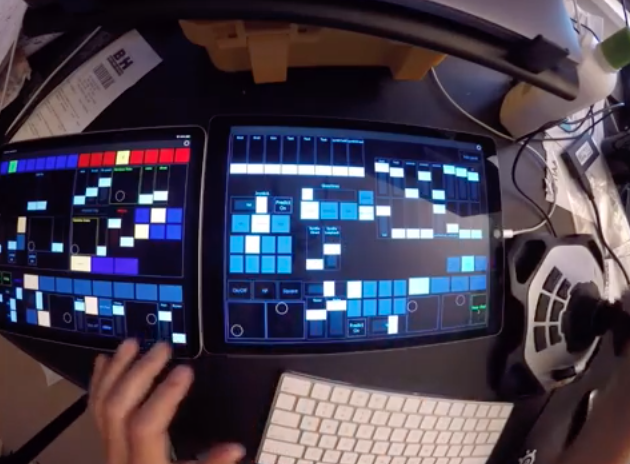
Pluta's two favoured controllers.
These shall be mapped to synthesizers:
- On the one hand we have the DX7 synths which Pluta describes as “really soupy”.
- On the other we have the cross feedback synths which are much more jerky, cutting, and chaotic.
Pluta explained that he developed the various synthesizers with specific controllers in mind, while playing with that specific controller; he also describes, for example, how the xy pad naturally “makes sense with my fingers” when mapped to the DX7, and the same for the joystick and the cross feedback synth. There is clearly a cybernetic feedback loop between HID, synth, mapping, and the way all of these things are conceived of in Pluta’s mind which is very difficult to disentangle.
It is important to understand this perspective when looking at Pluta’s instrument design. For example, when taken on its own, an HID is just a silent object with no inherently musical or interesting properties. Pluta discussed how, in his view, “all we have in electronic music are sliders and buttons”: he described cases where people can somewhat miss the mark when developing crazy controllers - at the end of the day, the interesting thing is how they will interact with the music. The important element is not the controller itself, but “how do you set up sliders and buttons in the way that allows us to be musically expressive?” The same can be said for the synthesizer – on its own it is just sound, there is nothing particularly interesting about it. It’s how it allows us to be musically expressive that is important.
Instrument design is ultimately about bringing things together in ways that allow us to be expressive. The powers offered by MLP regression allow for this to emerge from physical, immediate cybernetic feedback loops; they allow the instrument maker to quickly try things out, bring together dimensional mismatches in dynamic ways, and fluidly play, try, and embody configurations over the course of development.
Conclusion
We have seen how and why the MLP regressor was used by Pluta to empower his cybernetic instrument development system. To finish, let us discuss a further perspective that Pluta offered on instrumentality that englobes well many of the topics we have covered over the course of this article.
He explained that the reason he likes the joystick and the xy controllers so much, is because they are “slightly beyond my ability to comprehend where I am”. He went on to explain that for him, this is true with any instrument: “a flautist understands what they’re doing with their lips and their fingers, but I wonder if they could really describe physically what is happening when they play a certain multiphonic”. He explained that, in a book we can read the fingering of a multiphonic; however, 90% of the information is in the lips, embouchure, shape, how you’re blowing, the inner mouth, the posture of your face… This is almost impossible to talk or write about – it’s almost beyond comprehension. The flautist must intuit this to a certain extent.
This would seem to be a property that is very important in allowing for instrumentality in the nature of an object. He gave the example of a dual xy pad configuration: he cannot really picture that 4-dimensional space in his head when playing – but he can “totally intuit what [he’s] doing”. The 3-dimensional control space of the joystick is similar – straddling the line between comprehension of one’s actions and fuzzily navigating a space of too many dimensions to understand. He explained that this “allows you to be physical with the object and visceral with it, and have it still be surprising and exciting”.