
Exploring the Oboe with FluCoMa
In this article, we take a look at the work that Alex Harker did for the project, and how, in his piece Drift Shadow, he used the FluCoMa tools to explore the multiphonic possibilities of the oboe.
Alex Harker
Introduction
Download the demonstration patches for this article here.
Today we’ll be looking at some of the work that Alex Harker did for the FluCoMa project. We’ll be looking at how he took some of the tools and, in conjunction with his own library of Max objects FrameLib, used them to explore the instrument that constituted the acoustic part of the setup for his piece Drift Shadow: the oboe. The piece was co-created with oboist Niamh Dell who also performed to oboe part during the premiere. We’ll examine how Harker built a tool for oboe-following using an MLP classifier, and how the tools allowed him to navigate a large corpus of multiphonic audio as an aid for composition.
Drift Shadow, for oboe and live electronics, was premiered at the second FluCoMa concert as part of Dialogues Festival 2021 in Edinburgh. It was performed by Dell, and Harker was sat behind the desk, overseeing the electronics. The piece is characteristically emergent and flowing – gestures ease into each other. Time dilates and suspends itself as we are immersed within the ringing, delicate relationships of partials and complex microtones of the multiphonics. Things are simultaneously frozen and constantly shimmering; we are aware of a subtle interaction between the oboe and electronics which continually materialise from each other. With controlled fades and glissandi, the piece progresses through a series of intricate timbral textures that bring us into intimate proximity with the oboe.
It is a remarkable and complex piece. Upon listening, it is obvious that a very deep reflection around the timbral possibilities of the oboe’s multiphonics has occurred – both by the composer and the performer. We shall begin by discussing some of the elements that Harker wished to explore in this composition and what is happening on stage. Then we shall look at how he used the FluCoMa tools for Computer-Aided Composition (CAC), and how he approached MLP classification for tracking of the oboe.
Premise of the Piece
As is clear when listening to the piece, Harker explained that “the very starting idea of the piece was to explore the oboe from a timbral, multiphonic point of view, as an instrument that could create sound complexes rather than ‘notes’”. He cited the group Contest of Pleasures as being an influence for the piece, and the desire to interrogate ideas of techniques that are on the edge of control, and liminal sounds that split between various elements. He explained that “in the end it was really focused on timbre and texture in both the live [electronic]part and the instrumental part”: indeed, the way in which Harker approaches the multiphonic possibilities of the oboe is much less as ways of accessing a fixed set of notes, but as “fingerings that allow for a set of possibilities”.
An important aspect for Harker was also the amount of freedom that the performer has when performing the piece. This corresponds to the approach of multiphonics as allowing sets of possibilities: he explained that in this type of situation where the instrument is unstable and being approaches timbrally, he “wanted to give the performer some kind of freedom so that they’re not having to correspond to some kind of time measurement which is getting in the way of them responding to their instrument […] notating behaviours for the performer has always made more sense to me”. It is interesting to note Harker’s idea of the performer responding to their instrument. We shall explain this in further detail below, but the piece indeed allows for various types of freezing of the sound, and for prolonged interactions within those moments between the performer and the sound their instrument is creating.
Harker compared the piece to one of his earlier works, Fluence (which can be viewed in this video), where things are much more controlled. In Fluence, the structure of the piece is linear. In Drift Shadow, the computer is tracking what the performer is doing, and there is scope within the score for the performer to make decisions not only at a gestural level, but also on a more structural one. Harker explained that this kind of relationship between computer and player was interesting because of the possibilities for freedom it provides for the player. Indeed, he explained that detection “makes sense when you’re expecting things to be different”.
Harker openly states that the nature of the electronics in Drift Shadow is characteristically reactive: he has no intention to remove agency from the player and wishes for them to feel in control. For a larger discussion around this notion, you can take a look at the article about Hans Tutschku’s work for the project and the interactive/reactive polarity. Indeed, we have with Harker and Tutschku two slightly different approaches to a same notion of instrument-following – both technically (Harker uses MLP classification, Tutschku uses NMF seeding) and aesthetically. Before taking a closer look at how this works, let us first gain a better understanding of what exactly was happening on stage during the performance.
How it Works
The configuration in stage is somewhat typical for acoustic instrument and live electronics: Dell is playing into a microphone, the signal of which is being fed into a Max patch. There is a small monitor on stage that gives Dell feedback as to which section of the piece the electronics believes it is in, and she also has a foot pedal which allows her to lock into certain sections. We see that Harker is indeed giving the player control over the system and makes sure that they are aware of what the electronics are doing.
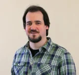
A page from the score for Drift Shadow.
Dell is reading from a remarkably beautiful score. Harker used the software LilyPond to produce the score which is far from being standardly linear and includes many bespoke symbols and notations that are all explained in extensive documentation at the beginning. In the image above we see the page that corresponds to the beginning of Part I, and notice the various arrows that give indications of possible progressions between different elements, multiphonic fingerings, slashes that indicate different ways of approaching playing, ways of visualising multiphonics etc. For a full explanation of what the various symbols mean, you can consult the beginning of the score which has been provided with the example patches.
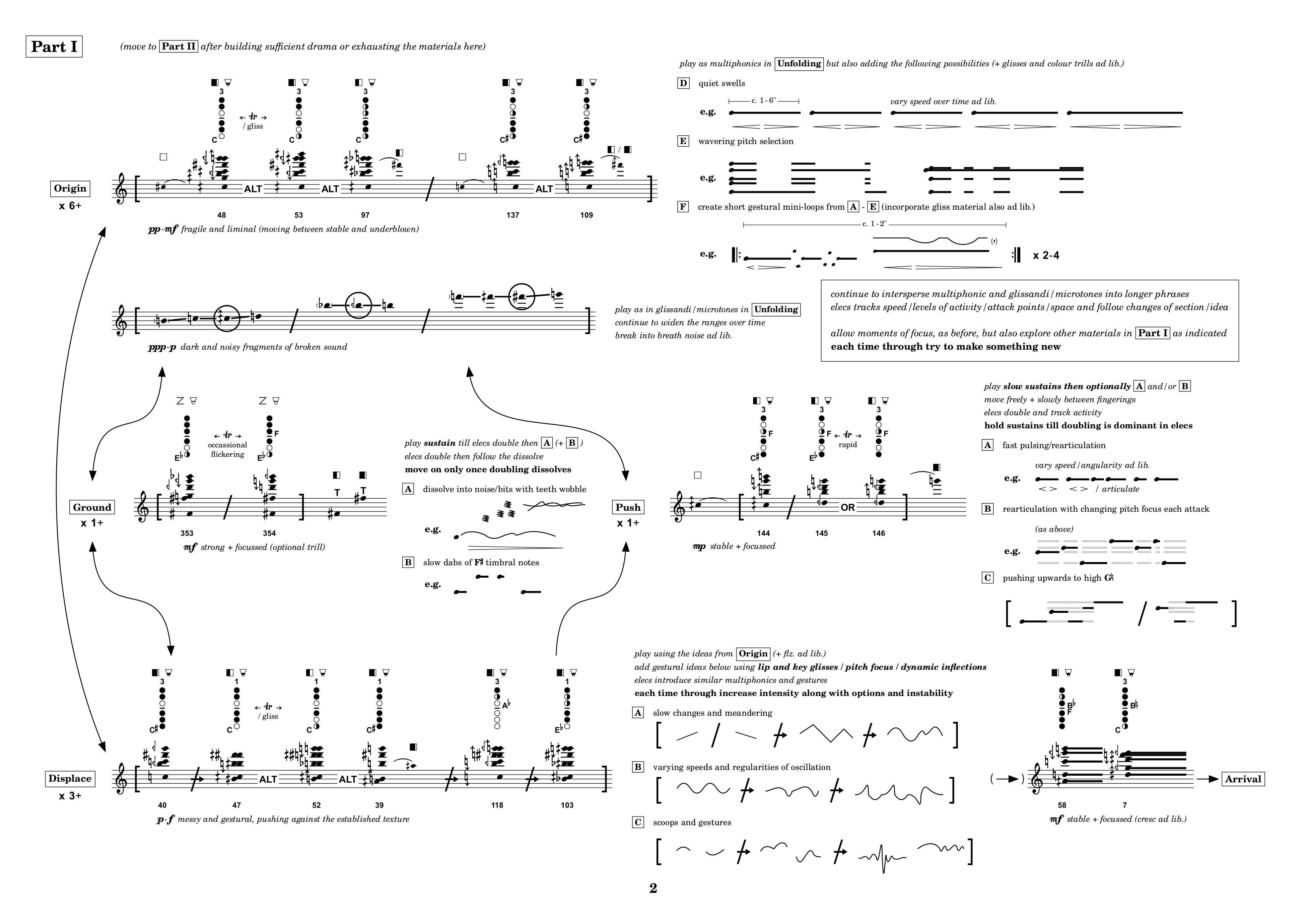
Overview of the software for Drift Shadow.
The whole of this score, with its various sections, conditional progressions, and rules, is also represented within the software. Indeed, the electronics are essentially divided into two elements, the first of which is the tracking of what the oboe is doing and deducting where in the score the performer currently is. We shall look at this in more detail below but let us first take a look at the other part of the electronics which is the various DSP techniques.
As you can see in the diagram, the main DSP techniques are various approaches to ‘freezing’ the oboe sound: spectral freeze, partial freeze, and granular freeze. They are all sample/playback based and depend on the tracking of the oboe multiphonics to be accurate in order to play back to correct content. Some of these techniques are implemented using Harker’s FrameLib objects. FrameLib is a DSP library for frame-based processing. Within Max, the user can create ‘networks’ – parts of the patch which happen within the FrameLib environment. These networks perform operations on groups of samples, the sizes of which can vary freely. The depth and scope of this library is immense, therefore if you are interested in learning more, we advise you download the tools and go through the excellent tutorials which are provided with them.
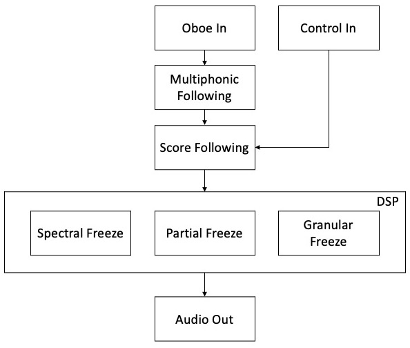
Example of a basic FrameLib network.
Harker implements his granular freeze with FrameLib, as well as his spectral freeze which is based on the stochastic phase vocoder example from the FrameLib documentation. The partial freeze takes the incoming multiphonic and resynthesises it through either sine waves or filtered noise. There is also scope within these modules for gestures between different voices that can all be controlled to a very fine level of granularity. For this article, we shall be focusing on the parts of the software that use the FluCoMa tools directly, but it is important to know that these freezing processes are what constitute a large part of the identity of the sounds emerging from the electronics. Again, if you wish to learn more about Harker’s approach to this kind of DSP, we recommend taking a look at the FrameLib documentation. Let us now take a look at the way Harker used the FluCoMa tools in conjunction with FrameLib in order to explore and track the sonic scope of oboe multiphonics.
Sample Exploration and CAC
Harker worked closely with Dell when developing the piece to explore the multiphonic possibilities of the oboe. A valuable resource for this was Peter Veale’s book The Techniques of Oboe Playing which lists over 400 different multiphonics with their corresponding fingers and embouchure. Harker described a first, laborious process of listening to recordings of all of these in order, saying that this was unsatisfying and not very productive. Indeed, it is understandable that listening to a series of 400 strident oboe multiphonics could be seen as somewhat of a hinderance for creative stimulation.
Download a small collection of oboe multiphonics recorded by Harker, performed by Dell here.
Harker needed a way to better navigate this large corpus of sounds, so he looked towards some of the FluCoMa tools – notably those for dimensionality reduction. This can be viewed and experimented with the example path 01 UMAP Corpus Explorer. In the image below we see on the right part of the screen the kind of sound plot that this technique is designed to provide. Each point in the plot represents the recording of a multiphonic, and their distribution in space will have some kind of meaning. The user can click around the space to hear the different sounds. This kind of data visualisation is similar to software like IRCAM’s CataRT, however the two axes here are not user-defined: they are derived from dimensionality reduction.
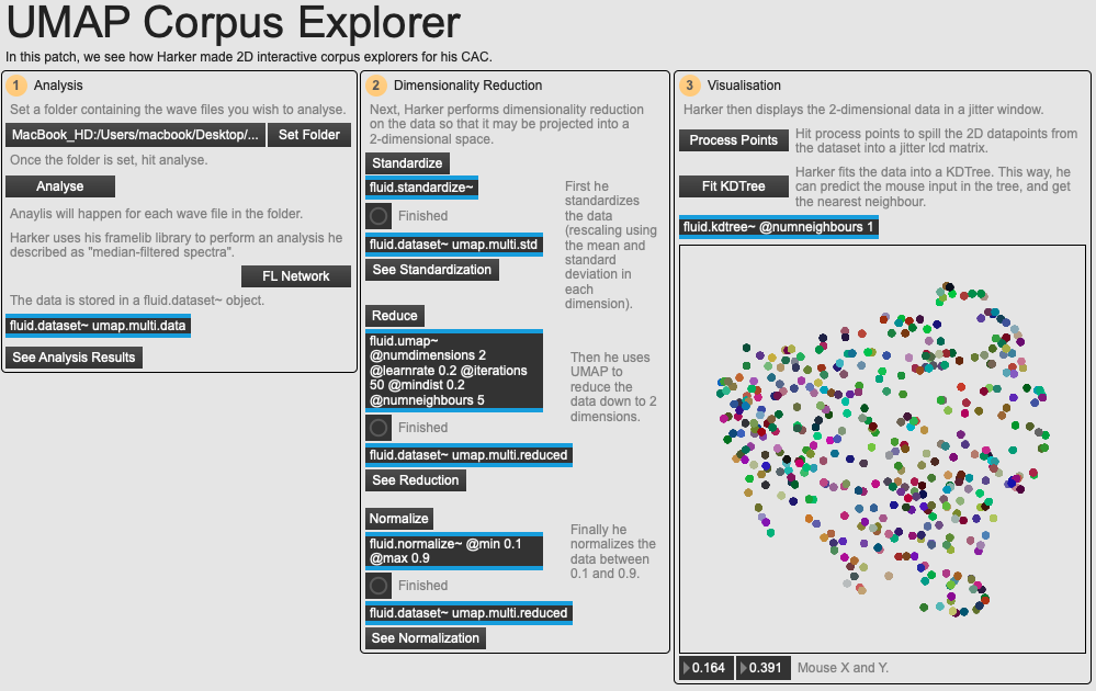
An overview of the example patch 01 UMAP Corpus Explorer.
Dimensionality reduction will consist of taking a large dataset – in this case, a collection of sounds that each have a large number of audio descriptor values (dimensions) – and crunching these dimensions down into something more manageable (for example, 2 dimensions which allows us to map these values to a visual 2-dimensional interactive interface). As you can imagine, there is no essential meaning to these resulting axes – however, the idea is that points that are close to each other in this 2-dimensional space will all have similar characteristics.
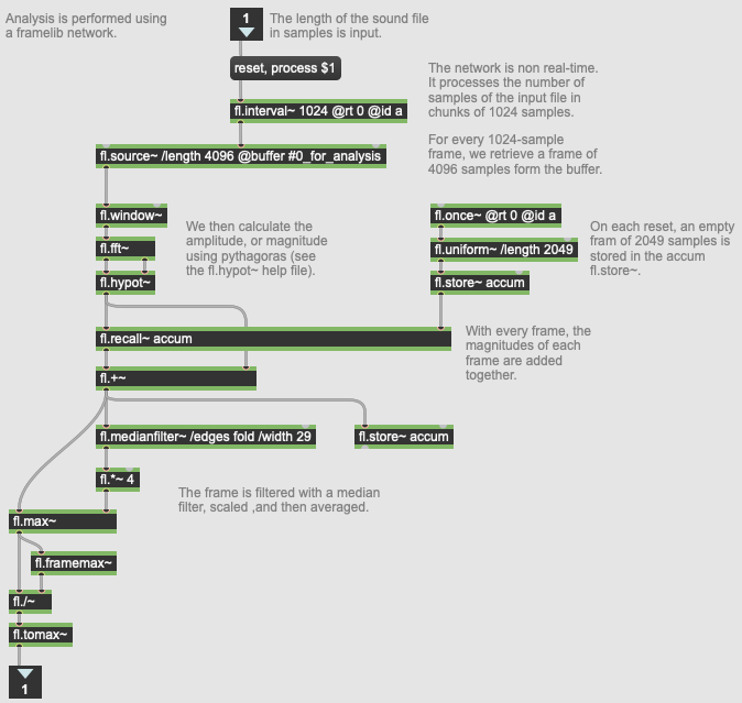
The FrameLib network used for analysis in 01 UMAP Corpus Explorer.
This also depends on the type of data that is being input. Typically, in our Music Information Retrieval context, the data will be audio descriptor data (such as those implemented in the FluCoMa tools like spectral shape, loudness, pitch, MFCC, mel bands). Here, Harker has implemented his own audio analysis using a FrameLib network. This can be seen in the image above: Harker describes the data as a median-filtered spectrum. We shall note across the various example patches that this is the way in which Harker will typically tend to analyse his audio for classification.
Harker uses this FrameLib network to analyse all of the sound he wishes and stores them in a fluid.dataset~ object: each sound file has a total of 2049 dimensions. He then standardizes the dataset using fluid.standardize~, before performing dimensionality reduction down to two dimensions. He uses FluCoMa’s implementation of the UMAP algorithm using fluid.umap~: he also experimented with the two other implemented algorithms fluid.pca~ and fluid.mds~. He then normalizes this data with the fluid.normalize~ object, before using Jitter to visualise it in a 2-dimensional space.
This was a great way for him to explore the corpus. Not only did it allow him to get a good idea of the scope of timbral possibilities offered by the different multiphonics, but it also allowed him, for example, to quickly find alternative fingerings to multiphonics that would sound similar. He would also experiment with different setups of this system, for example taking one multiphonic, and combining it with others and analysing the resulting harmonics. This approach offered itself as a powerful tool for composing with a corpus so rich, complex and extensive as that of oboe multiphonics.
For those that would be curious on seeing exactly how this technique works, you can delve into the example patch, or follow along the in-depth tutorial series we have on the subject. Next, let’s see how Harker approached tracking this kind of material for performance.
Oboe Tracking
Harker used the fluid.mlpclassifier~ object for tracking of the oboe during the piece. The example patch 02 MLP Classification shows how the process of training and predicting with an MLP neural network works. As we see in Section 1 of the patch below, we first gather our data that will be used for training.
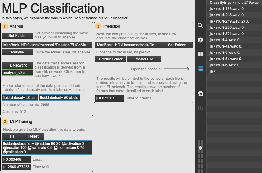
An overview of the example patch 02 MLP CLassification.
Once again, Harker uses a FrameLib network for analysis. Similarly, to the example discussed above, he retrieves the spectral magnitude, then performs the following operations:
- Thresholding based on a median filter (the filter gives a noise floor, and content below this is removed). This removes noise while retaining information pertaining to harmonics and partials.
- The frame is high pass filtered.
- The frame is compressed by raising it to the power of 0.6, and the normalized. This allows frames from a same fingering appear more similar to the neural network.
You can explore this FrameLib network in the example patch. This means that each file will be divided up into a large number of analysis frames, and these, along with their analysis results, are stored in a fluid.dataset~ object as datapoints. Harker also uses a fluid.labelset~ object to keep track of the different categories. Once analysis is finished, the user can fit the MLP classifier with this data as many times as they wish, trying to get the resulting loss down as low as possible.
Here we have simulated a system similar to the validation process that Harker used. You can run a file, or a whole folder of files against the MLP classifier, and the results will be posted to the Max console. The results show each of the different categories that were used to train the classifier, and the total of each of the frames of the prediction that were found to belong to that category. As you can imagine, in this example we ran the file multi-219.wav for classification, and as you can see, all 278 analysis frames were categorised with this label.
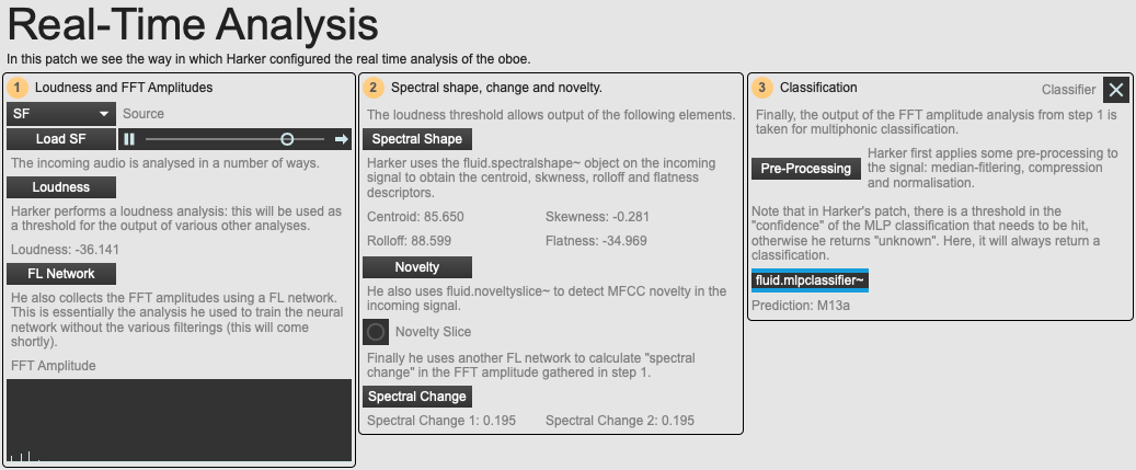
An overview of the example patch 04 Real-Time Analysis.
In example patch 04 Real-Time Analysis, we see how this classifier is used in the actual piece. This patch pre-loads with the training data that Harker used for the piece, and you can use the dry oboe recording of Dell’s performance as the analysis source. We see that with another FrameLib network, Harker is again retrieving the spectral magnitude of the signal and performing the same kind of pre-processing before predicting the data every analysis frame (every 2048 samples). We see that Harker also retrieves a whole host of other descriptor data – not all of them are used in the actual piece.
Harker wanted his oboe tracker to be fast – hence the tracking triggering with every analysis frame (roughly every 40ms). This was actually something that began to cause Harker problems: indeed, the fluid.mlpclassifier~ object is designed to always return an answer. However, Harker wished to find a way of only returning a classification if the neural network was sure about its prediction.
As you will have gathered from his extensive FrameLib library, Harker is an experienced programmer; he is no stranger to delving into the low-level depths of the Max CCE and programming his own externals. Along with FrameLib, he also has an extensive set of externals that perform a large scope of tasks that extend Max. Therefore, it is not surprising that, when faced with the issue in question, Harker decided that the simplest approach for him would be to go into the FluCoMa core C++ codebase, and recompile the fluid.mlpclassifier~ object so that it would behave in a way that would suit his needs (this code can be viewed here).
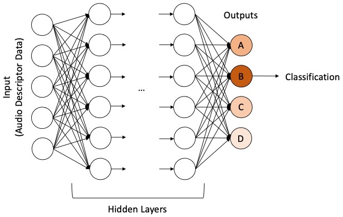
How an MLP classifier works.
In this diagram, we see a broad representation of how an MLP classifier works. Each of the different categories that were defined during training is represented as an output node. When inputting data into the neural network, each output node will have a certain value, a certain hotness – and the hottest node will be chosen as the resulting classification. Harker recompiled the object so that it would output not only this classification, but also the value of this hotness, and its ratio regarding all the other nodes. This meant that he could threshold output on these values, and if they were below the thresholds, the frame was classed as unknown.
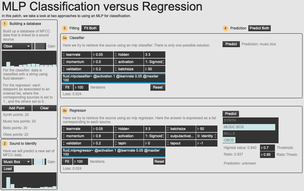
An overview of the example patch 03 Classification versus Regression.
It is possible to perform this kind of operation with the FluCoMa tools without resorting to this workaround. The solution is presented in the example patch 03 Classification versus Regression. Here, we see the same problem (classification of 4 types of sound source) being approached with two different objects: fluid.mlpclassifier~ and fluid.mlpregressor~. The classifier works in the same way as we have seen until now. The regressor works slightly differently but allows us to threshold the result in a way similar to Harker.
Instead of training the neural network by giving it a set of datapoints and their category, we train it by giving it the datapoints, and their categorisation as an array of numbers where the category = 1 and everything else = 0. So, for each datapoint representing classed as a synth, we give the output as 1 0 0 0, for music box 0 1 0 0 and so on. Now the output will be a list of numbers which are all mapped to a certain category.
Whatever way this is approached in practice, Harker explained that it was an essential step for increasing the accuracy of the classifier. In practice, there were a few other things that helped boost the classifier’s accuracy: for example, embouchure and tuning of the oboe was very important. Dell also played on the same type of reed that was used to train the MLP. Over the iterative process of development, she intuitively learned directions in which to push the intonation of certain multiphonics so that the computer would recognise them. Finally, Harker wrote the piece and the rules that allowed for its creation in a way that would avoid situations where similar sounding multiphonics would confuse the computer.
Conclusion
Drift Shadow takes a deep dive into the world of oboe multiphonics and creates a situation that allows the performer to explore this environment. We have seen how Harker took some of the FluCoMa tools and combined them with some of his own to allow for this. On a broader level, Harker explained that he saw this piece as a “step in the journey to a world that’s not sample playback, but not simple synthesis; where you get the complexity of real sounds but some of the flexibility about how you make them”. Indeed, he shares some of the primary goals with the FluCoMa project: to take a recorded sound and view it as a much more fluid thing; to be able to “free up a sound and do more things with it, but to keep its identity and character”. In Drift Shadow, not only does he take steps to achieving this with recorded sound, but also with the abstract sound world of a real, vibrating oboe and its player.