
Distribution and Histograms
Histograms, distribution functions, and the normal distribution
Histogram
Many of the statistical summaries that BufStats computes are intended to provide some insight on how the data is distributed across the range that it covers. A distribution is often approximated as a histogram, which divides the range covered by the data into discrete bins and then shows how many values in the data fall within each bin. The way a histogram ends up looking (and how informative it may be) is quite dependent on how many bins are used and their width.
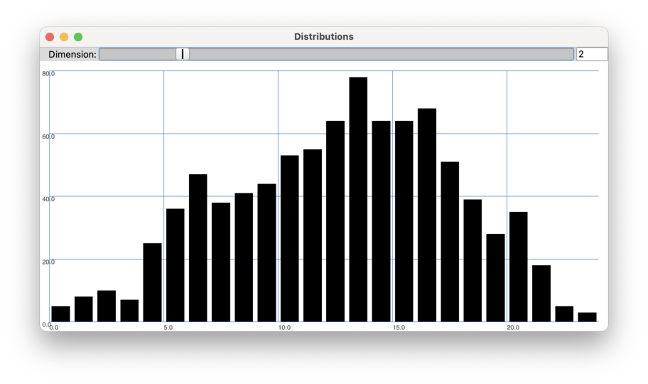
A histogram of 25 bins showing the distribution of MFCC 2 values in an analysis of Nicol-LoopE-M.wav
Sometimes the distribution is represented as a curve which can be called a distribution function. It shows the likelihood that a data point will exist for any given value in the range.
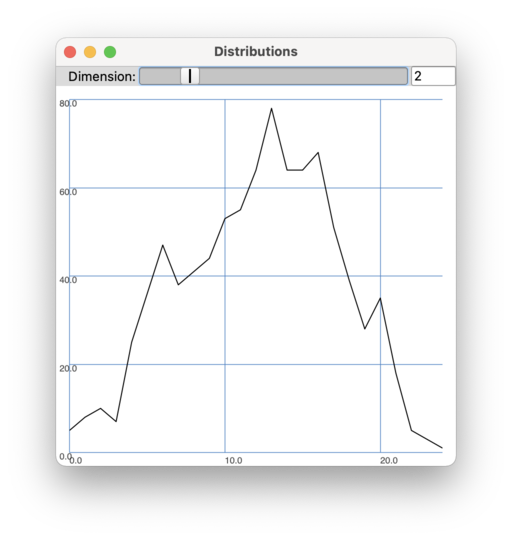
Distribution function based on the same data as the histogram above.
Keep in mind that the distribution functions are not the functions being analysed by BufStats, but instead represent the distribution of the values in the buffer channel being analysed by BufStats.
Normal Distribution
Normal distribution (also called a Gaussian Distribution) is a technical term meaning that the distribution of data demonstrates a set of certain characteristics.
- The mean, median, and mode are all coincident, meaning they are the same value.
- The distribution function is symmetrical around this coincident value.
- The data follows the 68/95/99.7 rule.
Sometimes a normal distribution is referred to as a “bell curve” because the shape of the distribution function looks like a bell. Use the example code below to see the distribution of dimensions in a dataset and how much they look like a bell curve.
The 68/95/99.7 Rule
If a collection of values is normally distributed, it follows the 68/95/99.7 rule. This rule states that ~68% of the data falls within one standard deviation of the mean, ~95% of the data falls within two standard deviations of the mean, and ~99.7% falls within three standard deviations of the mean. Because of this property, the mean and standard deviation taken together provide a lot of understanding about how the data is distributed.
For example if a SpectralShape’s spectral centroid time-series is analysed and BufStats returns a mean of 8000 Hz and a standard deviation off 1000 Hz, one can estimate that ~68% of the spectral centroids in that time series fall between 7000 and 9000 Hz (8000 Hz ± 1000 Hz). Similarly, one could estimate that ~95% of the data will fall between 6000 and 10,000 Hz (8000 Hz ± 2000 Hz) and ~99.7% will fall within between 5000 and 11,000 Hz (8000 Hz ± 3000 Hz). Keep in mind that if the data is not normally distributed, this will not hold true.
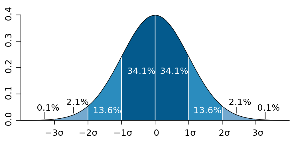
When data is normally distributed, it follows the 68/95/99.7 rule, indicating how much of the data is found within standard deviations of the mean. (image reproduced from Wikipedia)
Uniform Distribution
Uniform distribution indicates that any value within a range is equally likely to occur. Because of the shape of the distribution function, this is also referred to as a rectangular distribution. One place this is often seen is in a spectrogram of white noise, which contains equal power across frequency spectrum. Similarly, pseudo-random number generators are often designed to produce numbers in a uniform distribution across a specified range.
Although the uniform distribution is sometimes associated with randomness, it does not necessarily mean that the values in the dataset are random, it just means that they are uniformly distributed. For example, if one creates a dataset of pitch analyses using one recording for every note on the piano, the dataset will be uniformly distributed across the range of MIDI values 21-108 (this would be a discrete distribution, rather than continuous). A randomly chosen point from the dataset would be equally likely to have any MIDI value 21-108.
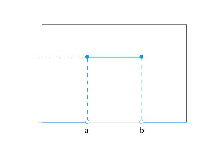
A uniform distribution function for the range of values between a and b. (image modified from Wikipedia)
Categorical Distribution
A categorical distribution describes the possible outcomes when a randomly selected variable may be one of K possible categories. The categories could be in any order but each will be in the range 0-1 (indicating a probability) and they will sum to 1. This can be seen when the Chroma argument normalize is set to 1, which ensures that all the Chroma values sum to 1. When used in this way, Chroma indicates the likelihood of the incoming signal to be each of the pitch classes.
Example Code to Check Distribution
Example code to check the distribution of dimensions in a DataSet using a histogram
~distributions = {
	arg dataset, numBins = 100;
	dataset.dump({
		arg dict;
		var data = dict["data"].values.flop;
		var histograms = data.collect{arg dim; dim.histo(numBins)};
		fork({
			var win = Window("Distributions",Rect(0,0,800,820));
			var plotter = Plotter("Distributions",Rect(0,20,win.bounds.width,win.bounds.height-20),win);
			EZSlider(win,Rect(0,0,win.bounds.width,20),"Dimension:",ControlSpec(0,histograms.size-1,step:1),{
				arg sl;
				plotter.value_(histograms[sl.value.asInteger]);
			},0,true,80);
			win.front;
		},AppClock);
	});
};