
BufStats
Statistical analysis of buffer channels
BufStats statistically summarises a set of values that are in a buffer channel, by returning seven statistics: the mean, standard deviation, skewness, kurtosis, low (by default the minimum), middle (by default the median), and high (by default the maximum) values. The mean and median are a measure of the central tendency of the data, while the others help describe how the data are distributed around this tendency.
A buffer typically holds time-series information as “frames,” either in the form of audio samples (as an audio buffer for playback) or as a series of audio descriptors created by an analysis process (as is the case with FluCoMa’s buffer-based analyses). If different time-series (such as sound slices) are all a different number of frames long, it may be difficult to compare them. The statistical summary provided by BufStats can be useful for comparing these time series (for example, the mean analysis value from one time-series can be compared to the mean analysis value from another time series even if the original slices are different lengths).
In addition to computing these statistical descriptions on the original buffer channel, BufStats can also:
- compute these statistics on up to two derivatives of the original time-series with the
numDerivsparameter - apply weights to the various frames to produce a weighted statistical summary using a
weightsbuffer - find and remove outliers frames with the
outliersCutoffparameter
While it can be difficult to discern how to use some of these analyses practically (i.e., what does the kurtosis of the first derivative of spectral centroid indicate musically?), these statistical summaries can sometimes represent differences between analyses that dimensionality reduction and machine learning algorithms can pick up on. Including these statistical descriptions in training or analysis may provide better distinction between data points.
The stats output buffer of FluidBufStats will have the same number of channels as the source buffer, each one containing the statistics of it’s corresponding channel in the source buffer. Because the dimension of time is summarised statistically, the frames in the stats buffer do not represent time as they normally would. The first seven frames in every channel of the stats buffer will have the seven statistics computed on the source buffer channel. After these first seven frames, there will be seven more frames for each derivative requested, each containing the seven statistical summaries for the corresponding derivative.
Mean
The average value of the data. This is calculated by adding up all the numbers and the dividing by how many numbers there are. The mean can be used to describe the central tendency of a set of values.
Standard Deviation
Standard deviation describes of the amount of variation within the data in relation to the mean, which implies that it may only be useful when the mean truly represents a central tendency of the data. A lower standard deviation indicates that the values are generally nearer to the mean, while a higher standard deviation indicates that many values are more spread out, further from the mean. Standard deviation is measured in the same units as the data itself.
Standard deviation could also help calculate where most of our data points can be found. For more information about the normal distribution and the 68/95/99.7 rule see the learn page on distribution and histograms.
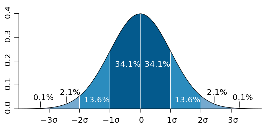
When data is normally distributed, it follows the 68/95/99.7 rule, indicating how much of the data is found within standard deviations of the mean. (image reproduced from Wikipedia)
Skewness
Skewness indicates asymmetry in the distribution of the data in relation to the mean. If the data is perfectly normally distributed, the distribution to the left and right sides of the mean will be mirrored, and skewness will be 0. If either side has a longer “tail” than the other, the skewness will not be zero. If the left side (lower values) have a longer tail, the skewness will be less than 0, if the right side (higher values) have a longer tail, the skewness will be greater than 0. The larger the tail, the larger the magnitude of the skewness value.
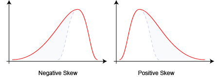
Data distributions with a larger tail to the left have a negative skewness while data distributions with a larger tail to the right have a positive skewness. (image reproduced from Wikipedia)
Kurtosis
Kurtosis describes the degree to which outliers are present in the data, sometimes described as whether the tails (extremities) are “light” or “heavy.” While a normal distribution has a kurtosis of 3, distributions with “lighter” tails (fewer and/or less extreme outliers) will be between 1 and 3, and distributions with “heavier” tails (more and/or more extreme outliers) will be greater than 3 (and can go up to infinity).
One can see in the image below that the pink rectangle-shaped distribution function has the lowest kurtosis (1.8) because it essentially doesn’t have outliers: all the data falls within range of the rectangle. The second lowest kurtosis (2) is the blue distribution function which also doesn’t have “tails” that spread out on either side. As the kurtosis increases (all the way to 6 for the red distribution function), notice how the tails end up being “heavier,” or “thicker” and can be seen to spread out farther beyond the mean.
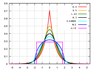
Kurtosis values (shown in the upper right hand corner) for various symmetric distributions. (image modified from Wikipedia)
Although, it doesn’t hold true for all data, kurtosis is sometimes described as the “peakedness” of a distribution. In the chart above, one can see how distribution functions with higher kurtosis are also “peakier,” while the distributions with lower kurtosis are “flatter.”
Order Statistics
The values returned as low, middle, and high are percentile values from the dataset (specified by the low, middle, and high parameters which can range between 0 and 100). A certain percentile is a value at or below which a that percentage of the values in the data will fall. For example, if the 15th percentile is 3000, that means that 15% of the values in the data are equal to or below 3000. The 50th percentile indicates the value which splits the data in half. This is also called the median. The 0th percentile will return the smallest value in the data and the 100th percentile will return the largest value in the data. These statistics are quite independent from the mean-related statistics above. Order statistics can be more robust when dealing with data that is strongly not normally distributed.
When the quantity of values does not make clear which point from the data should be used as a percentile, a nearest rank method is used, which ensures that the percentile values returned are always values actually found in the data. For example, for a set of MIDI values [ 60, 64, 67, 71 ] (a CM7 chord), asking for the median value without the nearest rank method would return 65.5, or F quarter-sharp, which is not in the chord! BufStats uses the nearest rank method and would return 67, a number that is actually in the data.
Low
The value returned will be the data point at the percentile indicated by the low parameter (between 0 and 100). The default of 0 will return the the smallest value in the data. It may be useful to use this statistical description to consider particular extremities in an analysis time-series. For example considering the smallest pitch confidence value in an analysis could indicate if there are any moments in the analysis that get unpitched and if so, to what degree.
Middle
The value returned will be the data point at the percentile indicated by the middle parameter (between 0 and 100). The default value of 50 will return the median value. The median is the middle value when all the numbers are sorted in order. This provides a measure of central tendency different from the mean. The median is not affected by extreme outliers, which can decrease how useful a mean is for understanding central tendency.
High
The value returned will be the data point at the percentile indicated by the high parameter (between 0 and 100). The default value of 100 will return the largest value in the data. It may be useful to use this statistical description for analyses in which the largest value has the most impact on a listener’s perception. For example, how loud one perceives a drum hit to be may be better correlated with the maximum loudness instead of the mean loudness, which will be brought down by the quieter parts of the decay tail and any silence that exists in the sound slice.
Derivatives
Setting the parameter numDerivs > 0 (the maximum is 2) will return BufStats’ seven statistics computed on consecutive derivatives of the channel’s time-series. The derivative of a time-series is approximated by finding the difference between each consecutive value in a series, which helps in understanding how a time series changes throughout time.
A musical example
Derivatives can indicate how a time-series (of an audio descriptor for example) changes over time. Consider the two sounds below. The top one is a snare hit with its loudness analysis overlaid. The bottom is the same snare hit but reversed. The mean Loudness for both of these is about -33 dB, therefore it’s not useful to distinguish the two. Looking at the derivative can help. In the top chart one can see that the change between adjacent loudness measures tends to be negative (go down), so the derivative will be mostly negative numbers—and therefore the derivative mean will be negative. In the bottom chart, the change tends to be positive (go up), so the derivative will be mostly positive numbers—and therefore the derivative mean will be positive. Sure enough, the mean derivative for the top chart is -0.8 dB and the mean derivative for the bottom chart is 0.9 dB. These numbers can now be useful in distinguishing these two sounds.
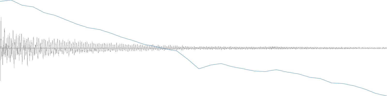
A single snare hit and its loudness analysis.
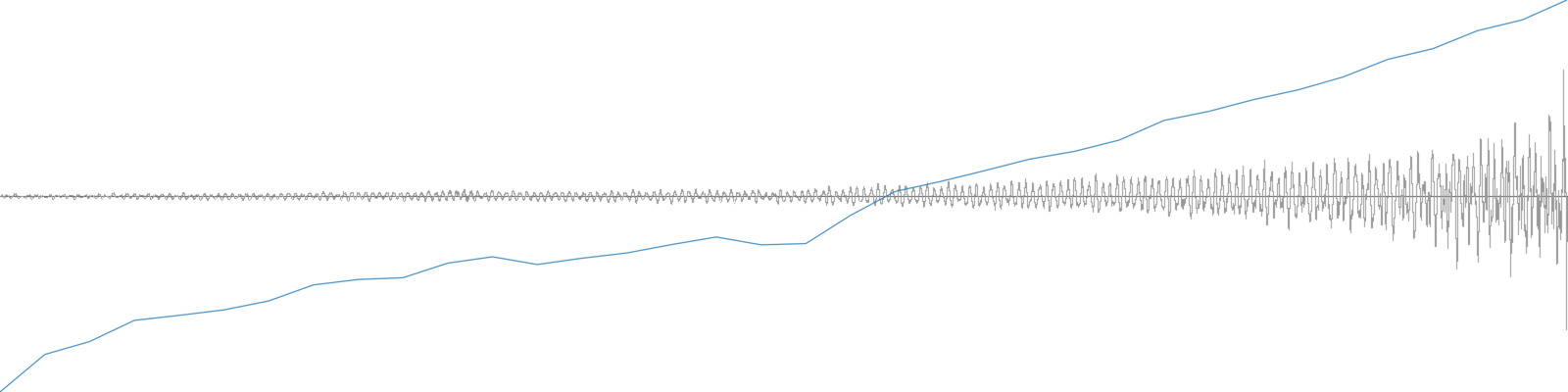
A reversed snare hit and its loudness analysis.
Approximating Derivatives
The derivative of a time-series is approximated by finding the difference between each consecutive value in a series. For example, the derivative of the input time-series in the top row is seen in the bottom row:
| A time-series and it’s derivative | |||||||||
|---|---|---|---|---|---|---|---|---|---|
| Original Time-Series | 10 | 15 | 30 | 20 | 25 | 12 | 0 | 24 | 40 |
| First Derivative | 5 | 15 | -10 | 5 | -13 | -12 | 24 | 16 |
Note that the derivative has one fewer value than the original series because each value represents the amount and direction of change between two adjacent values in the original. To find the second derivative, BufStats computes the derivative of the first derivative:
| A time-series and two derivatives | |||||||||
|---|---|---|---|---|---|---|---|---|---|
| Original Time-Series | 10 | 15 | 30 | 20 | 25 | 12 | 0 | 24 | 40 |
| First Derivative | 5 | 15 | -10 | 5 | -13 | -12 | 24 | 16 | |
| Second Derivative | 10 | -25 | 15 | -18 | 1 | 36 | -8 |
After computing the number of derivatives indicated by the user, BufStats calculates the same seven statistical summaries on these new series of numbers: mean, standard deviation, skewness, kurtosis, low, middle, and high.
Outliers
BufStats can find and remove outliers by using an analysis of the data to set boundaries for each channel in the buffer. Any frames that have a value outside the its channel’s boundaries will not be used to compute the statistics. The strictness of these boundaries is determined by outliersCutoff (see the page on outliers to learn more).
Weights
The weights parameter can be passed a buffer, the values of which will be used for relative weighting of each corresponding frame in the source buffer. This will create “weighted” statistics where some values in the data have more impact on the resulting statistical summary than others. All seven of the resulting statistics may be affected by using the weights.
This can be useful for weighting certain moments in descriptor time-series by the value of other descriptors. For example, one might want to weight the influence of pitch analyses using the pitch confidence descriptor so the resulting mean pitch value is more strongly influenced by moments in the analysis when the pitch confidence is high. Similarly, one might want to weight a descriptor time-series (such as MFCC) by amplitude so the louder moments of the sound slice have greater impact than the quieter moments on the resulting statistical summary.
For an example of using a weights buffer to influence the statistical summary in a musical way, visit the Weighting Stats Overview.
Not providing a weights buffer will cause all the frames to be considered equally. Any negative values in the weights buffer will be treated as a weight of 0. The provided weights buffer must be a single channel with exactly the same number of frames as source (each frame in weights will be the weight amount for the corresponding frame in source).