
OnsetSlice
Onset detection with various spectral slicers
Introduction
OnsetSlice calculates slice points in a sound based on changes in its spectrum. It makes these judgements based on one of several available metrics, which each have their own characteristics. From this, it derives a time-series that describes change from one moment to the next. If that change exceeds the given threshold parameter, a slice point for that event is produced. Let’s break this process down step-by-step visually.
A Visual Example
Let’s first start with this vocal recording:
If we create a spectrogram from this sound, it is visually explicit where significant changes in the spectrum occur. Aligning these visual differences, they seem to coincide with the utterances of each letter from the alphabet.
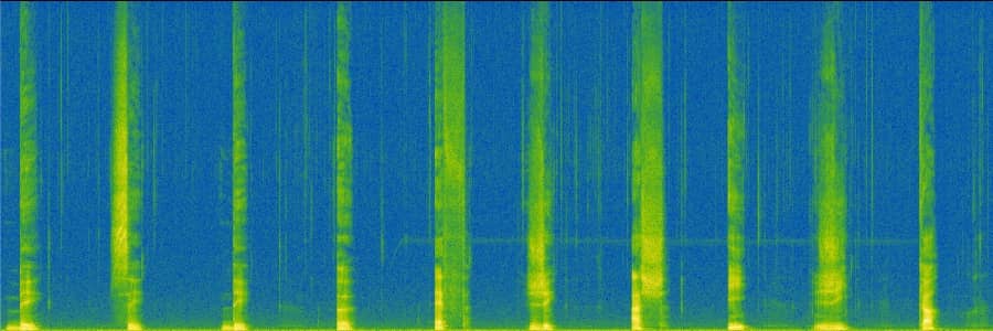
Spectrogram of Tremblay-AaS-VoiceQC-B2K
OnsetSlice measures change in this spectrum (according to its metric) and constructs a feature curve of its own. Points in time when the value of this curve exceeds the threshold are considered as onsets. Furthermore, another condition has to be met: the previous value must be less than the threshold. Below is an interactive widget that lets you visualise adjusting the threshold (the horizontal red line) and how this results in the detection of time slices (the vertical red lines). We used metric 2 to create the feature curve.
Metrics
There are 10 different metrics that OnsetSlice can use for calculating the changes in the spectrum. It can be overwhelming to know which one might be best for each scenario, and in many cases it might be a red herring to experiment with the metrics blindly. In all cases, we highly recommend starting your experimentation with metric 9. It works well with a wide range of sounds and has a normalised threshold range, meaning you only need to experiment with values between 0.0 and 1.0. Another good choice is metric 2. For more details read below, and most importantly, experiment using your ears in your creative coding environment of choice.
Metric 0 (Energy)
Difference between sum of squares of the magnitude of frames. Good for material that has large differences in amplitude.
Metric 1 (High Frequency Content)
Similar to metric 0 except that each frequency bin is weighted by the bin number. This means that the high frequency content is weighted more strongly in the calculation of difference.
Metric 2 (Spectral Flux)
Measures difference between the magnitudes of spectral frames. A popular algorithm and a suitable choice for a variety of sound types.
Metric 3 (Modified Kullback-Leibler)
Similarly to metrics 6, 7, 8, 9, metric 3 compares a projection of the spectrum based on frames in the past and compares the reality to this projection. Importantly, this uses log magnitudes per bin, whereas most other metrics don’t.
Metric 4 (Itakura-Saito)
Uses the Itakura-Saito divergence to measure the difference between the past spectrum and an approximate projection from thatinto the future. For more information, see the wiki article.
Metric 5 (Cosine)
Calculates the difference between spectral frames using cosine distance.
Metric 6 (Phase Deviation)
Phase deviation uses past spectral frames to projects what the next frame from those will be. It then compares the projection to the reality. If the difference between projection and reality exceeds the threshold, a slice is output. This is especially useful for sounds which alternate or change between stable and unstable sonic states. An example of this might be sinusoidal or tonal material that rapidly becomes noisy.
Metric 7 (Weighted Phase Deviation)
Very similar to metric 6, except the phase is weighted by the magnitude.
Metric 8 (Complex Phase Deviation)
The same as metric 6 but calculated in the complex domain.
Metric 9 (Rectified Complex Phase Deviation)
The same as metric 8 but rectified.